---
title: "Quantifying radiation"
subtitle: "UV, VIS and NIR "
date: 2024-07-15
author: "_missing_"
contributor: "Lars Olof Björn, Andy R. McLeod, Pedro J. Aphalo, Andreas Albert, Anders V. Lindfors, Anu Heikkilä, Predag Kolarz, Lasse Ylianttila, Gaetano Zipoli, Daniele Grifoni, Pirjo Huovinen, Iván Gómez, I. and F. López Figueroa"
date-modified: today
---
::: callout-note
# First edition authors
{{< meta contributor >}}
:::
::: {.hidden}
$$
\newcommand{\Chem}[1]{{\mathrm{#1}}\xspace}
\newcommand{\Unit}[1]{{\mathrm{#1}}\xspace}
\newcommand{\mymu}{\mu}
\newcommand{\um}{\Unit{\mymu m}}
\newcommand{\ulitre}{\Unit{\mymu l}}
\newcommand{\ms}{\Unit{m\,s^{-1}}}
\newcommand{\umolflow}{\Unit{\mymu mol\,s^{-1}}}
\newcommand{\umol}{\Unit{\mymu mol\,m^{-2}\,s^{-1}}}
\newcommand{\molms}{\Unit{mol\,m^{-2}\,s^{-1}}}
\newcommand{\umolt}{\Unit{\frac{\mymu mol}{m^2\,s}}}
\newcommand{\umolnm}{\Unit{\mymu mol\,m^{-2}\,s^{-1}\,nm^{-1}}}
\newcommand{\mmol}{\Unit{mmol\,m^{-2}\,s^{-1}}}
\newcommand{\mmolt}{\Unit{\frac{mmol}{m^2\,s}}}
\newcommand{\mol}{\Unit{mol\,m^{-2}\,s^{-1}}}
\newcommand{\ppm}{\Unit{\mymu mol\,mol^{-1}}}
\newcommand{\ppmt}{\Unit{\frac{\mymu mol}{mol}}}
\newcommand{\mmolmol}{\Unit{mmol\,mol^{-1}}}
\newcommand{\mmolmolt}{\Unit{\frac{mmol}{mol}}}
\newcommand{\molday}{\Unit{mol\,m^{-2}\,d^{-1}}}
\newcommand{\kjday}{\Unit{kJ\,m^{-2}\,d^{-1}}}
\newcommand{\kjhour}{\Unit{kJ\,m^{-2}\,h^{-1}}}
\newcommand{\kjdaynm}{\Unit{kJ\,m^{-2}\,d^{-1}\,nm^{-1}}}
\newcommand{\kjmole}{\Unit{kJ\,mol^{-1}}}
\newcommand{\jsecond}{\Unit{J\,s}}
\newcommand{\msecond}{\Unit{m\,s^{-1}}}
\newcommand{\Js}{\Unit{J\,s}}
\newcommand{\watt}{\Unit{W\,m^{-2}}}
\newcommand{\wattcm}{\Unit{W\,cm^{-2}}}
\newcommand{\wattt}{\Unit{\frac{W}{m^2}}}
\newcommand{\wattsr}{\Unit{W\,sr^{-1}\,m^{-2}}}
\newcommand{\wattnm}{\Unit{W\,m^{-2}\,nm^{-1}}}
\newcommand{\mwattnm}{\Unit{mW\,cm^{-2}\,nm^{-1}}}
\newcommand{\mwattmnm}{\Unit{mW\,m^{-2}\,nm^{-1}}}
\newcommand{\wattcmnm}{\Unit{W\,cm^{-2}\,nm^{-1}}}
\newcommand{\gmcubic}{\Unit{g\,m^{-3}}}
\newcommand{\irr}[1][]{{E_{\mathrm{#1}}}\xspace}
\newcommand{\sirr}[1][]{{E_{\mathrm{#1}}(\lambda)}\xspace}
\newcommand{\pfd}[1][]{{Q_{\mathrm{#1}}}\xspace}
\newcommand{\spfd}[1][]{{Q_{\mathrm{#1}}(\lambda)}\xspace}
\newcommand{\quantum}[1][]{{q^{\mathrm{#1}}}\xspace}
\newcommand{\molequanta}{\quantum[\prime]}
\newcommand{\flrat}{\irr[0]} % fluence rate
\newcommand{\PAR}{{\mathrm{PAR}}\xspace}
\newcommand{\PPFD}{{\mathrm{PPFD}}\xspace}
\newcommand{\RAF}{{\mathrm{RAF}}\xspace}
\newcommand{\eeff}[1][]{{s_{\mathrm{#1}}}\xspace}
\newcommand{\seeff}[1][]{{s_{\mathrm{#1}}(\lambda)}\xspace}
\newcommand{\qeff}[1][]{{s_{\mathrm{#1}}^\mathrm{p}}\xspace}
\newcommand{\sqeff}[1][]{{s_{\mathrm{#1}}^\mathrm{p}(\lambda)}\xspace}
\newcommand{\intensity}[1][]{{I_{\mathrm{#1}}}\xspace}
\newcommand{\radiance}[1][]{{L_{\mathrm{#1}}}\xspace}
\newcommand{\exposure}[1][]{{H_{\mathrm{#1}}}\xspace}
\newcommand{\dose}[1][]{{H^{\mathrm{#1}}}\xspace}
\newcommand{\sdose}[1][]{{H^{\mathrm{#1}}(\lambda)}\xspace}
\newcommand{\qdose}[1][]{{H^{\mathrm{#1}}_\mathrm{p}}\xspace}
\newcommand{\sqdose}[1][]{{H^{\mathrm{#1}}_\mathrm{p}(\lambda}\xspace}
\newcommand{\rad}[1][]{{L_{\mathrm{#1}}}\xspace}
\newcommand{\trans}[1][]{{\tau_{\mathrm{#1}}}\xspace}
\newcommand{\strans}[1][]{{\tau_{\mathrm{#1}}(\lambda)}\xspace}
\newcommand{\absb}[1][]{{A_{\mathrm{#1}}}\xspace}
\newcommand{\abst}[1][]{{\alpha_{\mathrm{#1}}}\xspace}
\newcommand{\sabst}[1][]{{\alpha_{\mathrm{#1}}(\lambda)}\xspace}
\newcommand{\refl}[1][]{{\rho_{\mathrm{#1}}}\xspace}
\newcommand{\srefl}[1][]{{\rho_{\mathrm{#1}}(\lambda)}\xspace}
\newcommand{\emitt}[1][]{{\epsilon_{\mathrm{#1}}}\xspace}
\newcommand{\SZA}{{\theta}\xspace}
\newcommand{\TOthree}{{\omega}\xspace}
\newcommand{\degree}{{\mathrm{^{\circ}}}\xspace}
\newcommand{\voltage}[1][]{{U_{\mathrm{#1}}}\xspace}
\newcommand{\temperature}[1][]{{T_{\mathrm{#1}}}\xspace}
\newcommand{\Coscor}{{\varphi}\xspace}
$$
:::
```{r, include=FALSE}
library(dplyr)
library(photobiology)
library(photobiologyWavebands)
library(photobiologyPlants)
library(photobiologyLamps)
library(photobiologyLEDs)
library(photobiologySun)
library(photobiologySensors)
library(ggspectra)
library(patchwork)
library(knitr)
```
## Introduction to radiation measurement
In this chapter guidance is given on how to measure and how to
interpret quantities describing the properties radiation, including the
application of the concepts of radiation physics presented in Chapter 2 to the
description and quantification of radiation in ways relevant to experimentation
in plant photobiology and the management of crops.
In research, When describing experimental conditions it is necessary to avoid
all ambiguity, so that current results can be interpreted correctly and
experiments reproduced. Expressions such as "light intensity" and "amount of
light", which are ambiguous, must be avoided. In addition, ambiguity must be
also avoided in equipment specifications and management recommendations targeted
at growers and other stakeholders. They depend on the information provided as a
basis for decisions affecting the success of their activities or even the
succesful implementation of government policies.
Instruments used to measure the properties of radiation are imperfect. All
measurements are subject to errors and uncontrolled variation. Some of this
variation is inherent to the individual instrument, including bias. However,
variation also occurs in response to other variables in the environment such as
temperature and humidity. In addition, the radiation-detectors used in some
sensors as well as electronic components used in the circuits that amplify and
record the measured quantities, age, i.e., their properties change with time.
Thus,to ensure accuracy and reproducibility, recalibration of instruments at
regular intervals is a must.
How the instruments are used, i.e., consistently following a correct measurement
protocol together with good awareness of the limitations of the equipment are
unavoidable requirements for accurate and reproducible measurements of all
properties of radiation.
::: callout-tip
# Accuracy and precision of radiation measurements
It is important to consider in each situation what are the required accuracy and
precision. When estimating changes in irradiance over long periods of time, instrument calibration drift is the most important source of bias. When
comparing measurements done with different instruments, the accuracy of their
calibrations and possible bias introduced by extraneous variables such as temperature are most important. These are the hurdles that meteorologists most
frequently have to deal with.
In a biological experiment were the different light conditions are measured with
the same broadband sensor, the main consideration is whether the calibration of
the instrument is valid under each light condition. When measuring a light
source at near range (up to several meters), using the correct distance between
source and sensor becomes crucial. When small differences among conditions are
more important than absolute values, precision is more important than accuracy.
Extraneous shading and reflections by objects and by the operator during
measurements can introduce very large errors haphazardly. Poor levelling of
diffusers, and in permanent installations, soiling of diffusers can also
become important sources of bias.
Replication in time and space are needed to quantify real-world variation. On
the other hand, the accuracy of calibrations is reported in calibration
certificates. This accuracy applies only to the calibration itself under the
conditions under which it was done, and weakens with differences in temperature
and with time. Sensor specifications sometimes include a description of the
dependency on temperature and in most cases recommended annual or bi-annual
recalibration.
It is also important to keep in mind that many instruments reach rated accuracy
only after a warming-up period. This applies also to artificial light sources,
including LEDs. They should be measured only after their temperature is stable
and obviously at the same temperature as when used.
It is worrying that in biological research these points are rarely taken into
full consideration, and almost never described in the methods section of
publications. _The clearer the description of the methods used
is in a reaserach paper and the more carefully measurements are done, the longer
the "shelf-life" of
a piece of research will be. This is in part because the longer the time since publication
what is not explicitly explained becomes more difficult for readers to fathom.
Fulfilling the requirements for reproducibility, makes research aoutcomes more likely to be cited in literture reviews and used in
meta-analyses increasing the long-term impact._
:::
A comprehensive glossary of terms relating to visible and ultraviolet radiation
has been published by @Braslavsky2007. It can be downloaded from the Internet
(see link in reference list).
After an introduction to the different types of instruments and discussing
generic features of measurement protocols including some caveats, the remaining
of this chapter is organized by physical and biologically relevant quantities,
starting from those covering the widest range of wavelengths. For each quantity
commonly used sensors and instruments are described together with specific
measurement protocols and common errors and pitfalls affecting them. Suppliers
known to the authors are also listed.
## Spectroradiometers {#sec:spectroradiometers}
Spectroradiometers measure spectral irradiance, usually expressed in
$\mathrm{W\,m^2\,nm^{-1}}$ or equivalent units differing only by a scaling
factor, e.g., $\mathrm{mW\,cm^2\,nm^{-1}}$. The wavelength resolution of
spectrometers can vary from a fraction of a nanometre to a few tens of
nanometres. What distinguishes data obtained with a spectroradiometer is that
radiation over a wide range of wavelengths is quantified at each of many ($\gg
100$) contiguous narrow wavelength "slices" or bands. Spectroradiometers are
spectrometers with entrance optics that makes it possible to measure irradiance
or, exceptionaly, fluence rate.
Spectrometers fall into two main groups: _array spectrometers_ based on an
array of detectors and a single static monochromator grating, and _scanning
spectrometers_ based on a single detector and one or two moving monochromators.
Within each approach there are different types of detectors in use, different
types of monochromators, and different optics. However, in some respects array
and scanning spectrometers are fundamentally different.
In array spectrometers the monochromator projects radiation of different wavelengths onto different sensors arranged as a linear (1-dimentional) array. Thus, the
whole spectrum is measured simultaneously. In a scanning spectrometer, the
moving grating projects radiation of different wavelengths sequentially
onto the same and only sensor. Thus, radiation at each wavelength "slice" is
measured at a different point in time.
Scanning spectroradiometers a based on a mechanism that accurately moves the
manochromator(s) in very small steps, in most cases motorised. Mechanical
accuracy and sturdiness depend on a rigid, and heavy structure. For this reason, scanning spectrometers are in general much bigger and heavier, and, thus, more
difficult to transport than array detector spectroradiometers. They
are also less tolerant to rough handling and vibration, and they usually require mains power. However, scanning spectrometers can accomodate a double monochromator
arrangement. The two monochromators are "in series" such that the light beam
passes through both of them before reaching the sensor. This improves markedly (by a few orders of magnitude)
the separation of light of different wavelengths reaching the sensor.
::: callout-note
The term _spectrometer_ is used to indicate that the same instrument, depending
on its attachments and calibration, can be also used to measure spectral
absorbance, -transmittance, or -reflectance, in addition to spectral irradiance.
:::
### Scanning spectroradiometers
THIS SECTION FOCUSES MAINLY ON THE SPECTRORADIOMETERS USED FOR LONG TIME
SERIES OF UV MEASUREMENTS IN METEOROLOGY. IT ONLY MENTIONS IN PASSING
SCANNING SPECTRORADIOMETERS FREQUENTLY USED BY BIOLOGISTS. THIS SECTION NEEDS
SOME EXPANSION AND REORGANIZATION. MENTION OR MANUAL INSTRUMENTS NOW NO
LONGER USED, COULD HOWEVER, WORK AS AN INTRODUCTION AS THEY ARE SIMPLER WHILE
BASED ON THE SAME PRINCIPLES. e.g. LI-COR LI-1800 from 1980's and ISCO SR from
1970's.
#### Basic structure and principles of operation
The basic components of a scanning spectroradiometer designed for fixed
installation outdoors are: a) input optics for collecting radiation from the sky
and guiding it further into the spectroradiometer b) a monochromator for
resolving the input radiation into separate wavelengths c) a photomultiplier
tube (PMT) or a solid state detector for sequentially quantifying the energy in
each spectral component of the measured radiation. In addition, scanning
spectroradiometers in most cases need to be used tethered to a personal computer
or tablet as they usually lack a built-in screen for user interface or enough
memory for data storage. EXAMPLE SPECTRORADIOMETER is needed here!! Biospherical and Brewer.
The input optics typically consist of a flat PTFE ("Teflon") diffuser disk
covered by a quartz dome. The diffuser collects the incident photons from the
overhead hemisphere. The resulting diffuse radiation is guided to the entrance
slit of the monochromator, sometimes by means of an optical fibre. The
monochromator may be a single or a double monochromator (see section
spectrographs). In scanning spectroradiometers, a system based on a step motor
drives a mask that allows only photons of a certain wavelength at a time to
enter the exit slit of the monochromator. The exit slit serves as the entrance
window to the cathode of the PMT. The photon pulses are amplified and
transmitted to a photon counter for registration.
While most frequently irradiance is measured on a plane parallel to the ground,
to measure "normal solar irradiance" spectroradiometers can be mounted on a solar
tracker that follows the position of the sun maintaining the plane of the diffuser
facing directly into the sun. A measurement head at the end of an optical fibre
may be also installed on a separate sun tracker. The temperature of the
instrument is usually either stabilized or kept above a certain temperature
limit to ensure proper functioning. The dome of the measurement head may be
equipped with a heater and/or air blower to keep the temperature of the teflon
within certain limits and to avoid formation of frost or dew on the dome
surface.
Scanning spectroradiometers intended for laboratory or spot measurements
outdoors are smaller and less rugged. They are more portable but more sensitive
to temperature extremes and are not water proof. Examples of such instruments
are Optronics OL 756 and Macam SR9910 spectroradiometers. Figure
[\[fig:Optronics:OL_756\]](#fig:Optronics:OL_756){reference-type="ref"
reference="fig:Optronics:OL_756"} shows the different parts of the first
of these instruments.
::: figure*
{width="0.9\\myfigwidth"}\
:::
The more rugged instruments, usually permanently installed at a fixed
location, are commonly used for measuring long (several years long) time
series of spectral irradiance data. The more portable instruments are
used for spot measurements in plant canopies, and under lamps, and or
filters. The first type of instrument is most commonly used by
meteorologists, while the portable instruments are most useful to
biologists.
#### Characteristics
**Dark current** and **dead time** are characteristics possessed by the
PMT. Dark current is a measure of the drift photons going from the
cathode to the anode of the PMT without any real incident photons
entering the instrument. Dead time is a measure of that PMT which is in
a paralysed state after a photon detection event. Stray light is
composed of photons reflected from wavelengths other than the nominal
wavelength being measured. In commercially available scanning
spectroradiometers, these phenomena are usually measured and handled by
the measurement software.
The **wavelength alignment** of a spectroradiometer has to be checked regularly.
Most instruments taking continuously sequential measurements contain an internal
mercury lamp aimed at ensuring the stability of the alignment. The wavelength
and the position of the micrometer turning the grating of the monochromator are
related to each other by a second-order equation using so called dispersion
coefficients. The determination of the dispersion coefficients should be part of
the annual maintenance of the instruments.
Solar irradiance spectra sometimes exhibit so called **noise spikes**,
which mean sudden abnormally high or low intensity readings on a single
wavelength. The origin of the spikes is not fully known, but
straylight is considered a partial explanation. The spikes can be
detected and eliminated making use of suitable reference spectra.
Ideally, the angular response of the measurement head follows the shape
of a cosine curve. In practice, the response deviates somewhat from
this. Typically, the larger the solar zenith angle, the larger the
deviation. The **cosine response** of the measurement head should be
measured in laboratory and a corresponding correction applied to
measured data.
If the spectroradiometer is not stabilized for temperature, its response
usually exhibits **temperature dependence**. This dependence should be
determined in the laboratory by measuring a calibration lamp with a
spectroradiometer heated/cooled over a range of different wavelengths.
The measurements can be used for deriving the temperature correction
factors to be applied in the post-processing of the sky measurements.
The **slit function** determines the transmittance of a monochromator as
a function wavelength. The ideal shape of the function would be
triangular. The full width at half maximum of the slit function is
commonly used as a quantity characterizing the slit function. The slit
function can be derived by measuring the irradiance emitted by a tunable
laser. Removal of the effect of the slit function on the measured
spectra should be considered if spectra measured by two or several
instruments are to be compared with each other.
The **spectral responsivity** of a spectroradiometer should be based on
regular measurements of a certified calibration lamp. If the
responsivity seems to have changed, basically two alternative ways to
handle the change exist. The change may be introduced in the
responsivity of the instrument and the processing of the sky
measurements as such. A step-wise change in response is hence introduced
in the time series of the measurements. Alternatively, a gradually
changing response time-series may be defined using a moving average with
a suitable time window. In this way, the change in the response is
introduced gradually in the time series of the sky irradiance
measurements.
#### Maintenance
The maintenance of a scanning spectroradiometer operating in an outdoor
environment involves the following practices: a) general daily
maintenance; b) checks on the wavelength setting and stability of
irradiance scale; c) calibration of irradiance against primary standards
in a dark room.
Daily routine maintenance includes cleaning of the quartz dome and
checking on the general functioning as well as the correct levelling of
the instrument. The quartz dome should also be cleaned/dried after rain
or snow. The operator should be familiar with the control software of
the instrument. Additional simple routines based on, for instance,
selected reference spectra may be used for instant checking of the
measured data. These kinds of routines are invaluable in the prompt
detection of occasional malfunctions of the instrument.
An internal Hg lamp is used for checking of the wavelength scale in some
spectroradiometers. In these cases, it is convenient to imbed the Hg
lamp measurement into the daily measurement schedule. If the instrument
lacks an internal lamp, this check has to be done using an external
lamp. For checking the stability of the irradiance scale, portable
calibration units are available. These enable, for instance, stability
checks of the instrument at the measuring site on a weekly basis. It is
advisable that the humidity indicators are also checked on a weekly
basis.
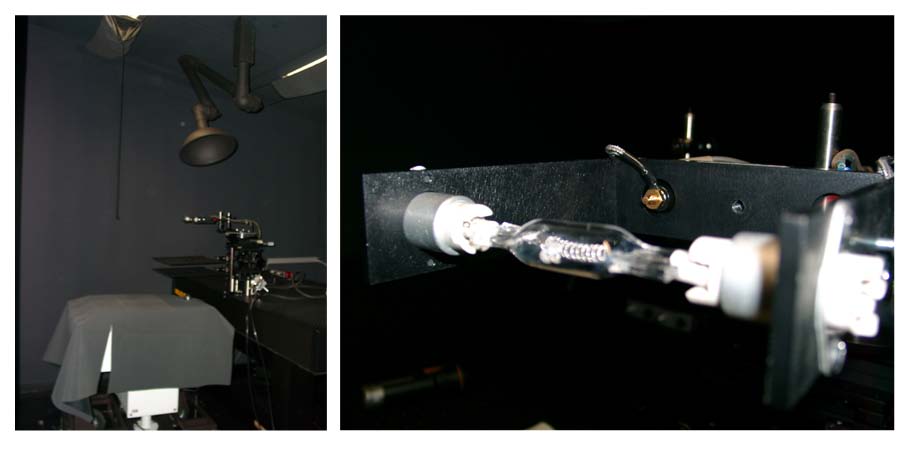
Irradiance calibration of a spectroradiometer should be performed in a
dark room (Figure
[\[fig:Brewer:calibration\]](#fig:Brewer:calibration){reference-type="ref"
reference="fig:Brewer:calibration"}). A primary standard lamp with an
irradiance certificate provided by a certified laboratory of standards
is needed. To extend the lifetime of the primary standard lamp, it is
recommended that it is not used as a regular calibration lamp. Instead,
the irradiance scale of the primary lamp should be transferred to a
secondary standard lamp that is used as a working calibration lamp. Use
of several working lamps is recommended to enable recognition of
potential drifts in the radiant output of the lamps as they age.
Calibration against the primary/secondary standard lamp should be
performed at least every two months. The desiccant bags inside the cover
of the spectrometer should be taken out and dried at least every two
months as well. Proper levelling of the instrument has to be ensured
after having it relocated for outdoor measurements.
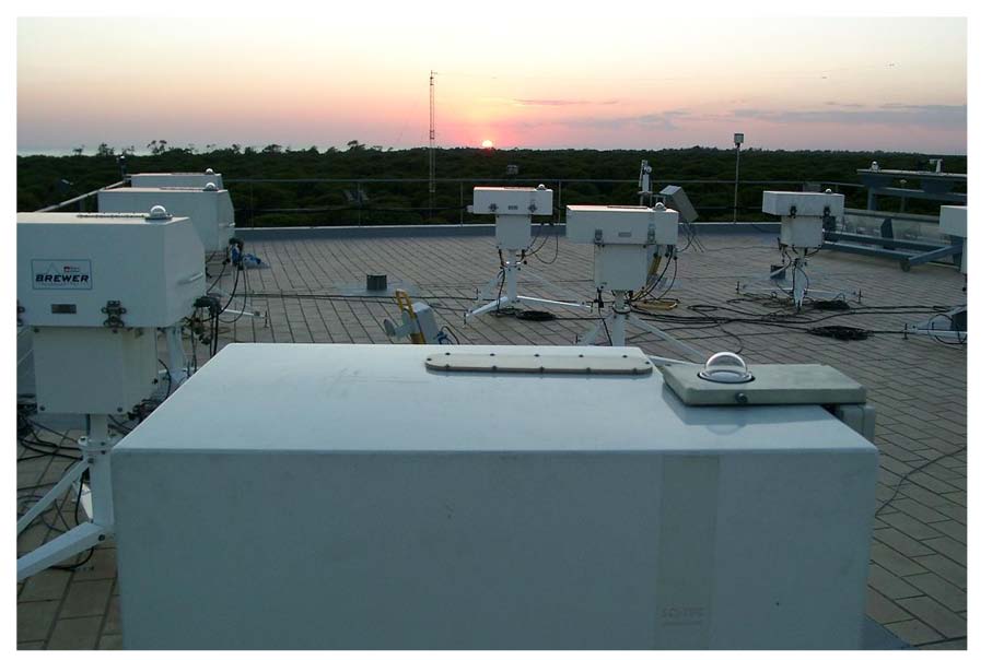
On the annual maintenance practices of a spectroradiometer, each
manufacturer has its own services and recommendations. Participation in
intercomparison campaigns gathering a number of state-of-the-art
instruments to conduct measurements on a jointly agreed schedule for a
period of time has proven a fruitful way to investigate the long-term
stabilities and overall performances of scanning spectroradiometers
(Figure
[\[fig:Brewer:intercomparison\]](#fig:Brewer:intercomparison){reference-type="ref"
reference="fig:Brewer:intercomparison"}).
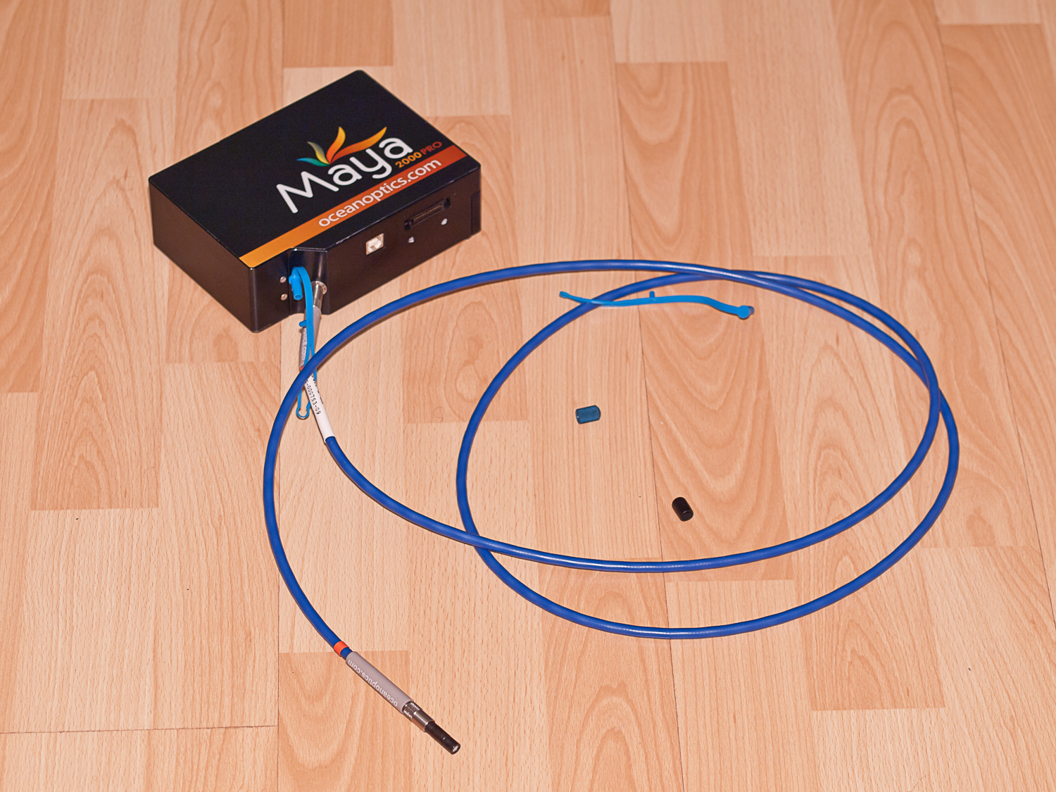
### Array detector spectroradiometers
In contrast to scanning spectrometers, array detector instruments
measure spectral irradiance simultaneously at all wavelengths. The
detector in this case is a linear array of light sensors, similar in
structure to the imaging sensors used in digital cameras, but long and
narrow. The number of detector elements ('pixels') along the array
varies, 2000 to 3000 pixels being common for visible light and fewer in
IR-only spectrometers. The array can be a
'charge coupled device' (CCD), or an array of photodiodes (DAD). The
'image' of the spectrum produced by the monochromator is projected and
focused by means of mirrors onto the linear detector array, each
detector in the array receiving light of a certain very narrow range of
wavelengths. In the
case of array spectrometers it is not possible to use two monochromators
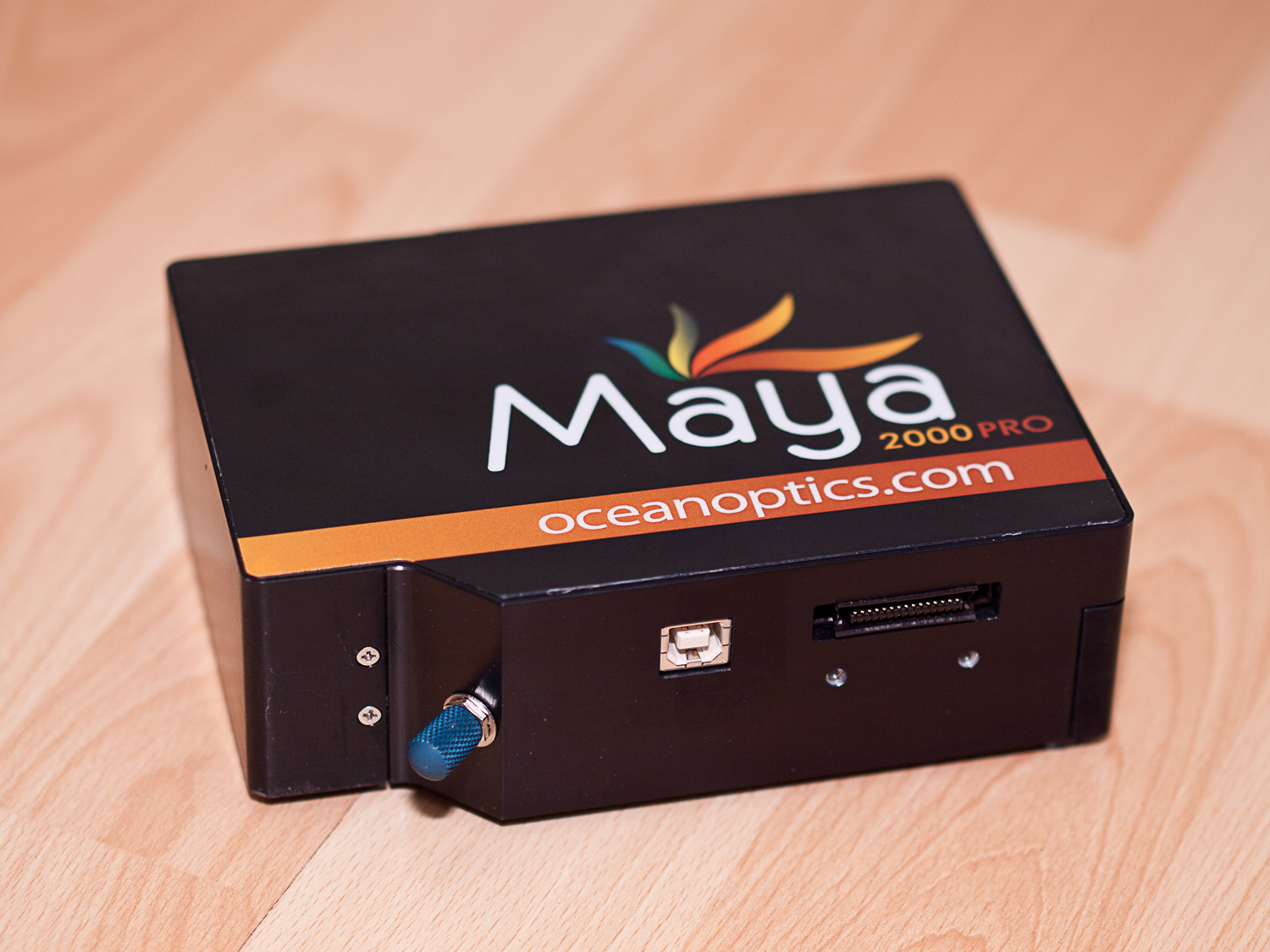
in tandem to reduce stray light. Array spectrometers are small and
portable (Figure
[\[fig:Maya2000Pro\]](#fig:Maya2000Pro){reference-type="ref"
reference="fig:Maya2000Pro"}).
For measuring energy or photon spectral irradiance a cosine diffuser is
used as input optics. This ensures that the angular response follows the
cosine law, and so the instrument measures the radiation as received on
a flat surface. Other input optics are also available, for example, with
a narrow angle of view. However, the quantity measured with them is not
irradiance. Cosine diffusers differ widely in how closely they follow
the cosine law. Some cheaper models are prone to large errors,
especially when radiation impinges at a sharp angle to their surface.
This will be further discussed in section
[9.7.2.1](#sec:array:errors){reference-type="ref"
reference="sec:array:errors"} on page .
The input optics is usually connected to the array spectrometer with an
optical fibre. The type of fibre to be used depends on the wavelength
range to be measured. If smaller than the entrance of the
spectroradiometer, the diameter of the fibre will affect the amount of
radiation entering the instrument. The diameter also affects the
mechanical properties of the fibre: thin fibres are more flexible and
tolerate bending into curves of smaller diameter. Fibres also vary with
regards to the type of cladding material used to protect them. Fibres
with metal cladding tolerate rougher handling than those with plastic
cladding. The most common connector for these fibres and accessories is
the SMA 905, originally designed for light fibres used in digital
communication systems. For this reason their positioning upon repeated
attachment is not exactly the same. Consequently, the recommendation is
**not** to detach and reattach the fibre from the spectrometer without
recalibrating the system[^24].
At the entrance of the spectrometer, just behind the connector to which
the fibre is attached, there is a slit (Figure
[\[fig:CCD:slit\]](#fig:CCD:slit){reference-type="ref"
reference="fig:CCD:slit"}), which limits the width and height of the
incoming light beam. The width is of the order of a few micrometres and
the exact value chosen determines, together with the monochromator, the
spectral resolution of the spectroradiometer. The narrower the slit, the
narrower the beam hitting the monochromator and the better the
resolution (the narrower the peaks that can be resolved). In a
Czerny-Turner configuration (Figure
[\[fig:optical:bench\]](#fig:optical:bench){reference-type="ref"
reference="fig:optical:bench"}), the next component is a collimating
mirror which projects the beam onto a monochromator. Gratings are used
as monochromators. Gratings have a surface with very closely spaced
rulings of a specific profile, and they separate radiation of different
wavelengths in a similar way to a prism. One important parameter is the
density of rulings which is one of the determinants of spectral
resolution and useful wavelength range. The 'image' produced by the
grating is focused onto the array detector by another collimating
mirror. Some newer models of spectrometer from StellarNet
(e.g. BLACK-Comet spectrometer) and now also from Ocean Optics (Torus
spectrometer) use a concave grating instead of a planar one. Since the
grating itself focuses the light onto the array detector, collimating
mirrors are not needed. Having fewer optical components, an instrument
with better stray light performance is obtained.
::: figure*


:::
::: figure*


:::
The array detector normally has rectangular 'pixels', orientated so that
their shorter dimension is on the axis along which the different
wavelengths have been separated by the monochromator, and their longer
dimension is perpendicular to it. The entrance slit is positioned to
have the long dimension coincident with the long dimension of the
pixels. In some detectors the long pixels are in reality rows of square
pixels with their electrical output combined into a single output
signal. The output signal from the pixels is averaged by the detector
itself over what is called 'integration time'. The longer the
integration used, the lower the irradiance that can be measured.
However, the 'dark noise' increases with the integration time. In
addition, it is possible to take several scans and average them. A
coarse dark noise correction is sometimes done by subtracting the signal
from special pixels at the end of the array that are not exposed to
radiation. However a dark scan, with the input optics protected from the
incoming radiation, should also be measured, and its value, wavelength
by wavelength subtracted from the measurements. The dark noise depends
on temperature. This has two implications, dark scans should be taken
frequently, sometimes before or after each measurement, and the
spectrometer should be allowed to warm up for some minutes before
starting to take readings. Furthermore, when working outdoors it should
be protected from direct sunlight, so as to keep its temperature stable
and close to that at which it was calibrated. Some spectrometers have a
thermoelement (TE), working according to the Peltier principle, which
cools the array detector to a preset temperature and thereby stabilizes
it.
Most array spectrometers, the exception being some older models with
thermoelectrically cooled detectors, are powered through the USB port.
This can be the same USB link to a personal computer used to control them
and retrieve the acquire spectral data. With the power delivery (PD) charging
protocol now available, USB-C ports can provide much more power that the
original USB 1.0 and 2.0 standards.
For field and mobile use a laptop is frequently used to control array
spectrometers. Special software, sold by the manufacturer of the spectrometer,
is frequently used to control the instrument and acquire and plot the spectra.
For most instruments there are also drivers and software development kits (SDK)
available for developing programs for special applications. When special
corrections, for example for stray light, are performed it may be necessary to
acquire raw spectral data and apply corrections and calibrations off-line using
other software, for example Excel or R. In some cases it is possible to control
spectrometers and acquire data using a microcontroller board such as the
Raspberry Pi.
Many modern array spectrometers can communicate through Ethernet in addition
to through USB. This makes it possible to control them through a local area
network (LAN) or through a wide area network (WAN) such as the Internet.
::: figure*
{width="0.67\\myfigwidth"}
:::
In recent years handheld array spectroradiometers have become available that
have a screen and small keyboard to control them. Nost of them are not designed
to measure ultraviolet or infrared radiation but only vsisible. Several of these
can be controlled wirelessly with a mobile phone through Bluetooth. Many of
these are not intended for or accurate enough for use in scientific research.
However, a few of them are. One example in the LI-180 from LI-COR. The
proliferation of suppliers of low cost spectrometers, frequently providing
incomplete descriptions and specifications, makes it hard to recommend any of
them for serious use, even if some could be fine and be available in the
future to provide support, repairs and updates.
#### Measuring errors and limitations in accuracy {#sec:array:errors}
Array spectroradiometers have a great advantage when quickly measuring
changing radiation as they acquire all wavelengths simultaneously. This
ensures that the values of spectral irradiance measured at all
wavelengths are consistent. In contrast, under conditions where
irradiance varies rapidly with time, the shape of the measured spectrum
can get badly distorted when measured with a scanning spectroradiometer.
However, array spectrometers have a serious limitation in that they
cannot be built with double monochromators. As any spectroradiometer
with a single monochromator, they suffer from relatively high values of
stray light. Stray light originates from scattered light of incorrect
wavelengths falling on a pixel of the array detector. In other words,
radiation of one wavelength is detected (and measured) as radiation of a
different wavelength. Perfectly scattered radiation would affect all
pixels in the same way, but when there are reflections within the
optical bench that are not perfectly scattered, some pixels in the array
detector are more affected by stray light than others. Stray light is a
critical specification when measuring UV-B in sunlight, as UV-B
irradiance is very low compared to the irradiance of visible and near
infra-red radiation. Consequently, if even a small proportion of visible
radiation is scattered and reflected as stray light within the
instrument, this stray light can generate a signal on the 'UV-B pixels'
of the array of a magnitude similar to, or larger than, that produced by
the radiation that we are trying to measure. Stray light is such a big
problem that without very complicated and special corrections these
instruments cannot be used at all to measure radiation in sunlight.
Errors of more than 100%[^25] for biologically effective doses can be
incurred even with a well calibrated instrument. Failure to take this
into account has led to important mistakes, like the erroneous
measurement of solar radiation at ground level by NASA researchers which
was published in *Geophysical Research Letters*. This was most likely an
artifact due to the limitations of the array spectrometer used. See the
paper by @DAntoni2007 and the refutation by @Flint2008 and the answer by
@DAntoni2008. Equally, the values of the UV-B doses used in many recent
biological experiments, as reported in the publications, are suspect,
since they have been based on measurements performed with
single-monochromator instruments.
Gratings disperse radiation according to what are called 'orders'. For
example first order dispersion may be 10 nm/mm, second order dispersion
5 nm/mm, third order dispersion 2.5 nm/mm, and so on. The first order
spectrum is what is of interest, and is what we want the array detector
to see. However, any given 'pixel' in the array, in addition to
radiation corresponding to the first order (e.g. 800 nm), also sees
radiation corresponding to higher orders (e.g. 400 nm, 266.6 nm, 200 nm,
and so on) if those wavelengths are present in the incoming radiation.
The solution to this problem is to use 'order-sorting filters' in the
light pass. In array spectrometers order-sorting filters may be directly
coated onto the array detector, or attached to it. For example Ocean
Optics spectrometers can be bought with a *variable longpass
order-sorting filter* as an option (Figure
[\[fig:CCD:slit\]](#fig:CCD:slit){reference-type="ref"
reference="fig:CCD:slit"}).
Another problem with array detector spectrometers is that the radiation
may be better focused on some parts of the array than on others, and
this causes changes in spectral resolution with changing wavelengths. In
addition, the wavelength difference between adjacent pixels is not
always the same across the whole spectrum, neither is the step size an
integer number. Usually the software supplied with the instrument can
generate files with data at integer steps (e.g. 1 nm, or 5 nm) but this
is done by interpolating and averaging, rather than changing the
measurement itself. In contrast the scanning step of scanning
spectroradiometers can be controlled through its software.
The overall accuracy of the measurements is also reliant on the angular
response of the entrance optics. For measuring spectral irradiance we
generally use a cosine diffusor as entrance optics, although it is also
possible to use an integrating sphere. Deviations of cosine diffusers
from the theoretical angular response tend to increase at large angles
from the vertical. If the spectrum of the light coming from different
angles is different (e.g. sun and sky) not only the irradiance measured
may be inaccurate but also the shape of the spectrum may be distorted.
When measuring outdoors, the size of this error will change through a
day as the sun moves across the sky. The very small cosine diffusers
sold by the spectrometer manufacturers tend to be prone to large errors,
and individually calibrated, high quality diffusers like the D7-SMA and
D7-H-SMA from Bentham (see section
[9.20](#sec:quant:suppliers){reference-type="ref"
reference="sec:quant:suppliers"} on page for full address) are
preferable, although they are much more expensive (Figure
[\[fig:Bentham:diffuser\]](#fig:Bentham:diffuser){reference-type="ref"
reference="fig:Bentham:diffuser"}).
::: figure*
{width="0.5\\myfigwidth"}
:::
#### Calibration and corrections {#sec:array:calibration}
When measuring UV-B with an array spectroradiometer it is not enough to
have it properly calibrated, its optical characteristics (slit function
at different wavelengths, stray light properties) need to be measured
and a correction algorithm developed and later applied to each
measurement. This makes the use of array spectroradiometers for
characterizing UV-B doses complicated and error prone. This type of use
has to be attempted only by experienced operators and the correction
algorithm itself requires lots of effort to develop and implement. Given
the lack of standardized procedures for stray light correction, its
implementation requires advanced knowledge of optics and metrology. We
will first discuss spectral calibration and thereafter stray light
correction procedures.
Spectral calibration against standard lamps needs to be repeated
regularly. For measurements not requiring very high precision, annual
re-calibrations may be enough. However, the main consideration should be
how valuable is the data that will be acquired. If the spectral
sensitivity of the instrument has changed significantly from one
calibration to the next, the data from all measurements done in between
these calibrations are suspect, and should be discarded. Consequently if
one does yearly re-calibrations one can lose one year's worth of data,
while if one does monthly re-calibrations one only risks losing one
month's worth of data. Consequently, the decision on how frequently to
calibrate should, in addition to instrument stability, be based on the
maximum size of the tolerable errors and on the value of the data
(i.e. the cost of replacing the data if they need to be discarded).
The most common and stable calibration light sources are incandescent
lamps (e.g. FEL lamps) with electronics in the power source which keeps
the electrical power at the filament constant within very narrow
margins. The distance between the lamp and the entrance optics, and
their alignment, should also fall within a very narrow margin of the
expected values. Calibration lamps are secondary or tertiary standards,
connected by a chain of calibration steps to a standard kept at a
metrology agency like NIST. Calibration lamps are supplied with spectral
data about their emission characteristics. Calibration of the instrument
is done by measuring the known spectrum and irradiance of the
calibration lamp. Of course the output of the lamp will not exactly
match the data supplied with it, because its original calibration is
also subject to errors. Furthermore, there are errors deriving from
slight differences between the burning conditions (current and voltage)
during measurements and those when it was calibrated at the factory.
Further errors can be introduced by small differences in the geometry of
the optical setup. So, do not forget that calibrations are subject to
errors. Furthermore, you cannot obtain an absolute estimate of
calibration errors by comparing two instruments calibrated with the same
lamp, unless this lamp is the primary standard.
Calibrating a spectroradiometer in the UV-B band with a FEL lamp is not
recommended, because FEL lamps emit very little UV-B. For calibration in
the UV-B deuterium lamps need to be used. Irradiance emitted by
deuterium lamps is less stable than that emitted by FEL lamps. For
coarse calibration the use of a deuterium lamp may be enough, but for
accurate calibration it is best to use FEL and deuterium lamps in
tandem. The shape of the spectrum emitted by deuterium lamps is stable,
by matching the irradiances at wavelengths where the emission of both
types of lamps overlap, one can extend an accurate calibration to
shorter wavelengths. Spectrometer manufacturers also sell calibration
light sources (lamp plus electronics) that may be good for routine
calibration or especially for checking that calibrations performed in an
optical bench remain valid. Again, what type of calibration procedure
and lamp to use will depend on the accuracy required. If we want our
measurements to be within $\pm 10$% of the true value we will need to
use very good equipment and protocols for the calibration. If we can
tolerate errors of, for example, $\pm 25$%, calibrations can be less
accurate.
It is also very important to do a wavelength calibration and to check
this calibration regularly. It should not be forgotten when doing this
calibration that it is affected by the temperature of the instrument as
temperature affects (by thermal expansion) the dimensions of the optical
bench and its components. Wavelength calibration is done based on
elemental emission lines in discharge lamps (or even the sun). For quick
checks low pressure mercury or germicidal lamps may be used. The
manufacturers of spectrometers also sell special light sources for
wavelength calibration. One should choose carefully which wavelengths to
use (for example 253.652 nm, 296.728 nm, 334.148 nm, and 404.657 nm for
mercury lamps, as they are simple peaks rather than multiple peaks very
close together like those at 302 nm, 313 nm and 365 nm). If one desires
a calibration accurate to a fraction of the wavelength step of the array
one needs to fit a bell-shaped curve to the pixel showing the highest
signal and those adjacent to it, to find the true location of the peak
centre, most likely in-between two pixels.
To keep errors within $\pm 10$% in the UV-B when measuring sunlight, and
especially to keep errors within $\pm 10$% for biologically effective
doses, a good calibration is not enough when using single monochromator
spectroradiometers. There is also a need to correct for stray light. If
we do not correct for stray light some biologically effective doses will
be overestimated by more than 100%. The ratio between stray light in the
UV-B band and the maximum spectral irradiance measured in good single
monochromator spectrometers is approximately 1$\times 10^{-3}$, while in
double monochromator spectroradiometers it can be as low as
$1 \times 10^{-6}$. If time for scanning, cost and lack of portability
are no obstacles, it's preferable to use double monochromator
instruments and these should also be used as the main instrument in a
laboratory.
When applying the stray light correction, a thorough characterization of
the slit function at different wavelengths and a check of the wavelength
dependence of stray light are needed. This characterization does not
need to be repeated, unless changes are made to the optical bench of the
instrument. So, in contrast to the spectral calibration, the stray light
characterization needs to be performed only once during the lifetime of
the instrument unless major repairs or modifications are made.
In some array spectrometers, depending on the configuration, the width
of the slit function may vary with the wavelength. This can introduce
errors that are very difficult to correct. In some cases it might be
preferable to chose a grating giving the instrument a relatively narrow
wavelength range, for example 250 nm to 500 nm if the intended use is to
measure ultraviolet radiation.
The use and calibration of array spectroradiometers for measurement of
UV-B radiation in sunlight is discussed in detail in the WMO report by
@Seckmeyer2010. Stray light correction methods are discussed in the
papers by @Ylianttila2005, @Coleman2008, and @Kreuter2009 and the
references therein.
## Broadband sensors
Broadband sensors in most cases measure irradiance in a single broad range of
wavelengths or band. Most broadband sensors used in plant research are based on
a photodiode, a filter to constrain the range of wavelengths reaching the
photodiode and a diffuser that provides an angular response close to that
proportional to the cosine of the angle of incidence of light over $\pm90^\circ$
from the normal, in three dimensions.
Not all broadband sensors measure irradiance: sensors with a different angular
response that proportional to the cosine of the angle are also available. Of
these, most common are those with a narrow aperture angle such as $\pm5^\circ$
from the normal. Spherical diffusers are used in aquatic sciences to measure
fluence rate and spherical irradiance. Least common are hemispherical diffusers
used to measure hemispherical irradiance or the fluence rate on a plane.
In traditional multichannel broadband sensors, such as red and far-red sensors,
each channel consists in a discrete photodiode and filter, with the channels
sharing the same cosine diffuser.
Not all broadband sensors rely on Silicon photodiodes. Some broadband
sensors are based of photodiodes made of other semiconductor materials such as
Silicon Carbide, Germanium, and Indium Gallium Arsenide. In addition, some
ultraviolet sensors rely on the secondary emission from an intermediate compound
to convert ultraviolet radiation into visible radiation that can be more easily
detected with Silicon photodiodes. These will be discussed later as the detector
choice depends on the wavelength band measured.
Although many broadband sensors simply provide the raw electric current from the
photodiodes as output, others have built-in amplification with a voltage output,
More recent designs include analogue to digital conversion circuitry and provide
as output through a digital interface. Nowadays, some suppliers even sell
multiple versions of each of their sensors, differing only in the interface used
to retrieve the readings. As these interfaces are unrelated to the measured
quantities, they are described here.
::: callout-warning
# Spectral response of broadband sensors
The spectral response of broadband sensors almost always differs to a larger or
smaller extent from that in the definition of the quantity being measured. The
consequence of this is that the calibration of any broadband sensors is not
constant, it varies depending on the spectrum of the radiation being measured.
In some cases these differences are so small that can be ignored, but in other
cases ignoring they can introduce large biases, invalidating the measurements.
In general the broader and more featureless radiation spectrum is, the less
likely a large bias is. In addition, some patterns of spectral response are technically easier to create than others.
**A very frequent and grave mistake is to assume _a priori_ that a calibration
provided by the sensor supplier, e.g., for sunlight is applicable to artificial
light sources, such as discharge lamps, incandescent lamps or LEDs.** Some
suppliers provide approximate correction factors (e.g., Apogee for sensor
SQ-301X-SS) or clear warnings in the documentation, while others do not even
warn users. In the case of sensors good enough to be used in research, suppliers
do provide _typical_ spectral response curves. Such curves are not guaranteed,
and should be taken with a grain of salt but can be used to estimate the
possible calibration errors. This does not replace a light-source specific
calibration.
:::
### Photodiode current
The electrical current generated by a photodiode is almost proportional to the
absorbed photons of a given wavelength, until its response saturates. The dark
current is extremely low. Thus, the best Si photodiodes show a linear response
over several orders of magnitude of irradiance. As the current depends on the
captured photons, the larger the area of the photodiode the higher the current
generated. The principle of operation is similar to that of solar panels used
for power generation. The diodes used in sensors have relatively small area and
the generated current is small, in the order of a few mA. Thus long wiring can
distort the signal or pick electrical noise from other devices. A sensitive and
accurate measuring device is necessary to measure medium and low irradiances.
Each sensor and sensor channel needs to be wired individually to a current
measuring device with a high enough impedance not to affect to the functioning
of the sensor. These sensors do not require a power supply and only two wires
needed between the sensor and meter or datalogger. The time constant of the
these sensors is very short, in some cases less that a ms and dependent on the
capacitance of the wiring.
### Amplified voltage
Some sensors have a built-in amplifier that converts the small current generated
by the photodiode into a voltage, commonly in $0\ldots 5$ V or $0\ldots 10$ V.
Unless the amplifier is very well designed, it can introduce a small zero offset
and introduce temeprature dependence. These sensors do require power for the
amplifier to operate. The wiring is less sensitive to electrical noise and a
measuring device of lower sensitivity and impedance can be used without
affecting the accuracy of the measurement. The time constant of the response of
these sensors vary as it is mainly dependent on the design of the built-in
amplifiers. It can vary from a few ms to 1 s or longer.
### Amplified current
Rarely used in research but frequently used in indutrial automation are
amplified sensor with a current output in the range $4\ldots 20$ mA. In this
protocol 4 mA corresponds to a zero reading. This relative high current makes
this type of wiring rather inmune to electrical noise. The drawback is that
these sensors consume more power than those using alternative approaches, making
them unsuitable for battery or solar-panel powered systems.
### Digitital communication
Digital communication protocols can provide two big advantages: the sharing of
wiring among separate sensors or between channels in a single sensor. As data
are transmitted as encoded numbers, their integrity can be checked. The most
frequently used wired protocol is SDI12 (serial data interface at 1200 bit s-1).
These sensors have built in circuitry for converting the current from the sensor
or the amplified voltage into a digital value. Many are also able to computed
time averages from individual measurements and keep the most recent value in
local memory. The "measuring" device, computer or logger, queries the sensor
for specific data and the sensor replies by sending a number encoded as train
of binary 0 and 1 plus a code to check integrity. Each sensor has an address
that identifies it within the sharing wiring and the logger or other measuring
device addresses its queries to a single sensor at a time. Multiple commands
can be implemented in a single sensor, even commands that change its behaviour.
It allows long wiring in addition to sharing it. Its drawback is that the data
rate is low, so data can be retrieved from sensors at most once every few
seconds. This time increases the more sensors share the wiring as they need to
be queried sequentially. Sensors implementing the SDI12 tend to be more
expensive than those based on simpler approaches. On the other hand they
remove the need to use loggers capable of accurate and high resolution analogue
to digital conversion.
In addtion to SDI12 other digital electrical and communication protocols are in
use for sensors. Two well-known serial protocols are RS-232 and RS-485. The
first of them is point to point with no sharing of wiring and it was common in
personal computers in the 1980's and 1990's. RS-232 even is data are sent serial
through a single pair of wires, acknowledgement and synchronization takes places
through additional wires. In RS-485, from around the same time, wiring can be
shared and addressing and coordination requires fewer wires. These are
electrical protocols. MODBUS is a comand protocol that uses RS485 and is still
in use, mainly in industrial automation but occasionaly also for tasks like
greenhouse automation and sensors.
### Miniature integrated sensors
A newer type of sensors, originally developed for use in mobile phones and TV
sets, are integrated circuits that have multiple photodiodes and the ancillary
amplification and analogue to digital conversion electronics built-in. They come
in SMD pacakages with footprints as small as $2\times 3$ mm. In some cases the
photodiodes have interference filters deposited directly onto the silicon chip
surface creating channels responsive to different wavelength bands. These
sensors are extremely small with all channels tightly clustered within an area
of the order of one to a few square millimetres. Some of these sensors can do
simple digital data processing to convert the measurements into physical or
photobiological quantities of interest. These sensors are designed to be paired
to microcontrollers and communicate with them using short-range digital serial
communication protocols and installed in devices. Ready to use devices,
specially weather-proof ones, are not yet commercially available. Some very
cheap handheld spectrometers are probably already based on these sensors,
although the suppliers do not disclose their design. Small modules including a
logger have been developed based on these integrated circuits. Also
instructions, breakout boards, code libraries are available for different
popular micro-controller-based boards like different flavours of Arduino,
Rasperry Pi and ESP32. Compared to traditional sensors these modules are much
cheaper and less accurate but still very versatile. For example the 14-channels
AS7343 spectral sensor from ams OSRAM sells for 7 € individually and much
cheaper in quantity. The USB module Yoto-Spectral from Yocto-Puce with
built-logger based on this same spectral sensor sells for 60 €. These sensors
are less accurate than traditional ones but the cost advantage is overwhelming
allowing high replication while the built in logger makes deployment easy.
### Wireless communication
There are multiple approaches to wireless transmission of sensor data. Some
rely on protocols widely used in other domains, such as Wifi, Bluetooth or
even GSM. In recent years the popularization of the internet of things (IoT)
has encouraged the development of protocols optimised for transmission of
sparse data from sensors, including LoRa and low throughput/low energy variants
of Wifi and GSM.
Selecting the wireless protocol to use depends mainly on necessary range, data
transmission throughput and the availability of power sources. The architecture,
meaning which data links are wired and which ones wireless can also vary. One
approach is to have individual sensors communicating wirelessly to a base
station where data are collected and possibly forwarded to remote storage
(e.g., Aranet's). Alternatively, multiple sensors can be wired to a hub and
the hub connected wirelessly to a router by Wifi, wired through ethernet or
through GSM or some other protocol.
## Data retrieval and logging
On-site data loggers with wired sensors is a common and relaible approach,
both at accessible and remote sites. Data are stored locally but in most
cases can be accessed locally, remotely or both. Data are normally downloaded
from the logger in batches. Modern loggers with ample memory can safely store
large data sets. Most loggers have an assortment of inputs, both analogue and
digital making it possible to attach sensors based on a mix of different
analogue and digital communication protocols. The best data loggers have
analogue to digital converters (ADC) with a resolution of 24 bits and auto
ranging. Some dataloggers like Campbell Scientific CR6 can take up to 100
readings per second simultaneously on more than one analogue input. They can
be programmed to take measurements only under certain conditions, compute and
store summaries like means and histograms instead of raw data, to power on and
off instruments and control ancillary equipment like cameras. Data loggers for
use in the field have been around for over 50 years and are a stable and
reliable, but expensive.
Small loggers, with only one or two channels and built-in sensors have been
available for some decades. Illumination loggers and PAR loggers are available.
Most of these sensors do not provide as good a performance as separate
sensors and loggers but are overall cheaper and easier to deploy, although
on site data collection from multiple loggers can become time consuming. The
iButton Thermocron temperature loggers in a button-cell-like case are widely
used, rugged and small. Nothing like them is available for measuring light.
PAR loggers are larger in size.
Some sensors with logging capabilities are also capable of being remotely
accessed. They provide the best of both worlds as data are locally stored
independently of any break in communication, but can be accessed remotely
to download the data, change settings or even update the firmware.
## Summaries based on wavelength ranges
The rest of this section is organized with one section for each group of
related measured quantities. In each of these sections the different
instruments and sensors and well as computations used to compute them from
spectral irradiance are presented.
### Global radiation and pyranometers
The term global radiation describes most of the radiation at ground level that
arrives from the sun, what in meteorology is called _shortwave radiation_,
extending from approximately 280 nm in the UV to nearly 2800--3000 nm in the IR.
Pyranometers measure radiation in this range as energy irradiance
($\mathrm{W\,m^{-2}}$).
Pyranometers are the most common radiation sensor used in meteorology, and
long-term time series of global radiation data from weather stations are
available. The best performing pyranometers use as sensor a blackened thermopile
(multiple thermocouples in series) enclosed to isolate it from the air and
external temperature changes. The thermopile behaves like a black body and warms
up in response to the incident energy flux. A difference in temperature between
the two sides of the thermopile generates a voltage difference approximately
proportional to the energy flux. The design ensures that radiation of nearly all
wavelengths in the global radiation range are nearly fully and equally absorbed.
Consequently, for radiation within the range 290 nm to nearly 2800 nm a single
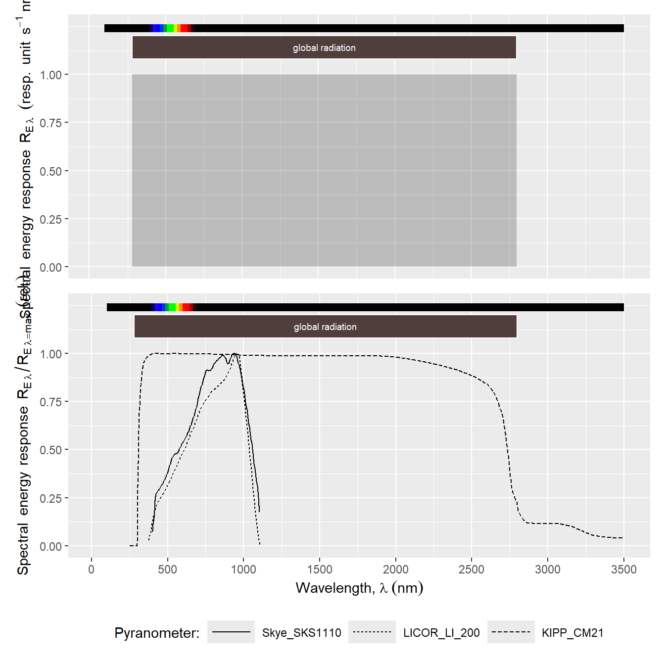
calibration is usually valid @fig-global-radiation-spct.
In contrast to most other radiation sensors, the spectral
response of thermopile pyranometers is in close agreement with the
theoretical quantity they are intended to measure. The performance of thermopile
pyranometers is described using standardised "classes", with each class having
different requirements for performance and accuracy. The current ISO 9060:2018
standard, calls the classes: A, B, and C, with required minimum performance
decreasing from A to C (formerly named "secondary standard", "first class" and
"second class"). Thermopiles in pyranometers are protected by one or two
concentric quartz domes. Some thermopiles used to measure radiation in
laboratories have more rudimentary or no protection. The best know supplier of
pyranometers is Kipp. The original design of the thermopile and domes has
remained nearly unchanged for decades. Versions with amplified and calibrated
voltage output, amplified current output as well as digital output have been
released more recently and coexist with earlier ones.
Cheaper "silicon" pyranometers work on a very different principle: a
semiconductor photodiode generates a current of electrons proportional to
absorbed photons. The response varies with wavelength not only because of the
varying energy per photon, but also because their quantum efficiency varies with
wavelength. The spectral response of these pyranometers is not flat with respect
energy or photon irradinace @fig-global-radiation-spct. In other words, there is
a mismatch between the spectral response of the sensor and the spectral
weighting of the physical quantity measured. _The consequence of this is that
sensor calibration is not independent of the spectrum of the radiation being
measured!_ This is also the case with most other broadband sensors based on
silicon-, silicon carbide-, and photodiodes made from other semiconductor
materials.
```{r}
#| label: fig-global-radiation-spct
#| fig-asp: 1
#| fig-cap: Comparison of the definition of global radiation to the spectral response of three pyranometers. The Kipp CM21 pyranometer is a thermopile-based instrument with an spectral response approximating the theoretical response. The Skye SKS1110 and LI-COR LI-200 are based on silicon photodiodes and even if their spectral response differs drastically from the expected one, they are calibrated to give a reading approximating global radiation **only** when used in sunlight.
global.wb <- waveband(c(280, 2800),
                      SWF.e.fun = function(x) {1},
                      norm = 550,
                      SWF.norm = 550,
                      wb.name = "global radiation")
autoplot(global.wb, range = c(100, 3500), geom = "spct") /
  (autoplot(sensors.mspct[c("Skye_SKS1110", "LICOR_LI_200", "KIPP_CM21")],
            idfactor = "Pyranometer:",
            range = c(100, 3500),
            annotations =c("-", "peaks"),
            w.band = global.wb) +
     theme(legend.position = "bottom")
  ) +
  plot_layout(axes = "collect")
```
Global radiation cannot normally be computed from measured spectral irradiance,
as spectrometers in common use do not have a wide enough wavelength sensitivity
range.
### Photosynthetic radiation and quantum sensors
Given the central role of photosynthesis, multiple radiation quantities to
quantify radiation that can drive the light reactions of photosynthesis have
been proposed over the years. A few competing quantities remain currently in
use. McCree's definition of the photon irradiance of photosynthetically active
radiation ($Q_\mathrm{PAR}$) is overwhelmingly preferred nowadays.
$Q_\mathrm{PAR}$ is frequently described as _photosynthetic photon flux density_
and abbreviated PPFD. PPFD is not used outside the plant sciences, "photon flux
density" widely accepted name is "photon irradiance" and its symbol is $Q$.
However, several other quantities can be found in the current and specially past
scientific literature on plant biology, plant ecology and meteorology. Some of
them, locationally, even under the same name "photosynthetically active
radiation" or PAR as McCree's.
Early on, given the availability of illuminance sensors, values expressed in
lux and foot candles were frequently used. In meteorology pyranometers, and
in Physics thermopiles, described above, have been in use for a long time, and
were also used to report energy irradiances. Both of these approaches are
inadequate and have been mostly abandoned in studies related to photosynthesis
and plant biology.
The earliest and simplest approach that considered the response to light of
photosynthesis was to constrain the range of wavelengths over which spectral
_energy_ irradiance was integrated to those contributing to photosynthesis,
however, with no agreement on the best range of wavelengths to use.
Spectral _photon_ irradiance can also be integrated over a wavelength range. As
described in chapter XXXX, the use of photon or energy as base of expression to
quantify radiation are not equivalent, and interconversion is only possible if
the light spectrum shape is known. As for any photochemically driven reaction,
absorption of photons excites chlorophyll molecules and this excitation energy
drives the chemical reactions. Thus, from a mechanistic perspective photon
irradiance should be preferred. Still in the early 1970's there was no consensus
and multiple ways of describing the radiation in studies with plants, including
photosynthesis, where in use. To make things worse, interconversion was in most
cases impossible as spectral information was not available @McCree1972a,
@McCree1972b, @McCree1976. McCree's proposal of PAR aimed to address this
problem, and was based on a large set of measurements of the spectral response
of photosynthesis.
In other words, PAR, as defined by @McCree1972b is the integral over wavelengths
of the spectral _photon_ irradiance
$$Q_\mathrm{PAR} = \int_\mathrm{400\,nm}^\mathrm{700\,nm} Q(\lambda)\ d \lambda$$
and is not directly equivalent to the _integral_ of the spectral energy
irradiance over the same range of wavelengths,
$$E_\mathrm{PAR} \neq E_\mathrm{PhR} = \int_\mathrm{400\,nm}^\mathrm{700\,nm} E(\lambda)\ d \lambda$$
where we $E_\mathrm{PhR}$ is photosynthetic energy irradiance as defined by
@Gabrielsen1940 and no longer in use in plant and agriculture research but still
used in meteorology, also under the name of PAR.
::: callout-note
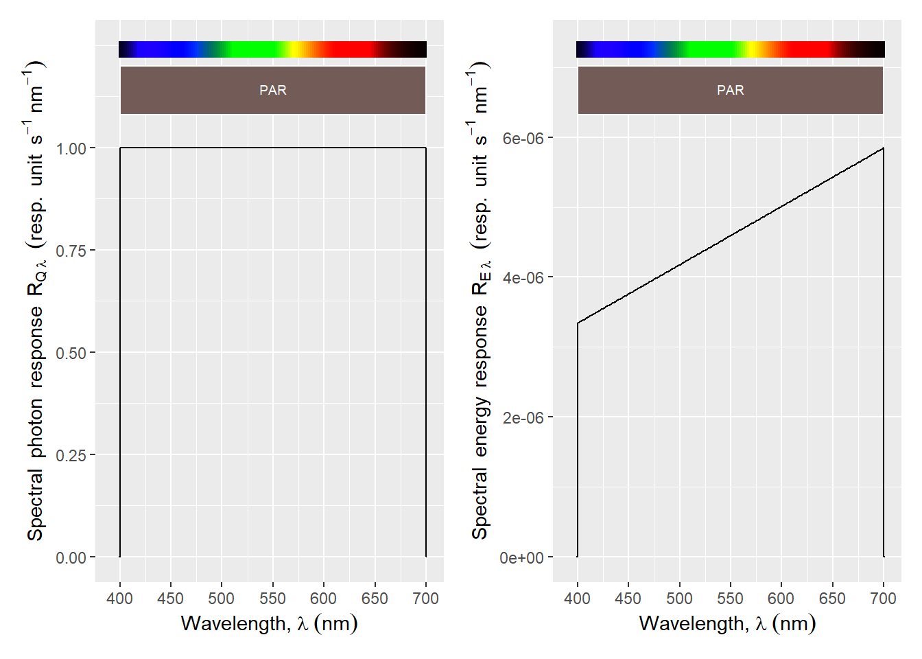
PAR as defined by @McCree1972b is based on a very simple biological spectral
weighting function (BSWF) according to which all photons in
$\lambda\ \mathrm{in} 400\ldots700\,\mathrm{nm}$ drive photosynthesis with
equal efficiency @fig-PAR-BSWF.
```{r}
#| label: fig-PAR-BSWF
#| fig-cap: The biological spectral weighting function (BSWF) of PAR as defined by McCree, plotted as normalised response per energy quantum (or photon) and per energy of incident light.
autoplot(PAR(), unit.in = "photon", unit.out = "photon") |
  autoplot(PAR(), unit.in = "photon", unit.out = "energy")
```
Thus, the PAR BSWF used with photon irradiance, is implicit in the equation above,
which could be written also as
$$Q_\mathrm{PAR} = \int_\mathrm{400\,nm}^\mathrm{700\,nm} a_q(\lambda)\times Q(\lambda)\ d \lambda$$
where
$$a_q(\lambda) = 1\ \forall\ 400 \leq \lambda \leq 700$$
That the action per photon is invariant with wavelengths implies that the
effectiveness of energy depends inversely on wavelength based on Plank's law.
This makes it possible to re-express the PAR BSWF in energy units.
However, the conversion is not unique, as it needs to be normalised based on a
reference wavelength. Below, $550$ nm, the wavelength at the centre of the
$400\ldots 700$ nm wavelength range, was chosen rather arbitrarily.
$$E_\mathrm{PAR} = \int_\mathrm{400\,nm}^\mathrm{700\,nm} a_e(\lambda)\times E(\lambda)\ d \lambda$$
where $a_e(\lambda) = \lambda / 550$ when using $\lambda = 550$ nm as
normalization wavelength for the BSWF.
The purpose of this explanation is to demonstrate that PAR is intrinsically
defined as a photon irradiance, not as a wavelength range as sometimes
erroneously assumed. PAR should always be
reported as a photon irradiance ($Q_\mathrm{PAR}$ = PPFD) and a different name
used for the energy irradiance $E_\mathrm{PhR}$, if used at all.
For sunlight, when using $\lambda = 550\,\mathrm{nm}$ for normalization, the
difference between $E_\mathrm{PhR}$ and $E_\mathrm{PAR}$ is quantitatively
rather small, but for some other light sources the difference is too large
to be ignored.
:::
The definition of PAR proposed by @McCree1972b was inspired by how illuminance,
the brightness of light as perceived by humans is routinely measured. He
proposed a definition based on numerous action spectra of photosynthesis he had
measured in leaves of several different crop plants. These action spectra were
based on absorbed photons rather than on the incident photon flux. He decided to
ignore the effect of variation in absorptance on the basis that absorptance is
very high in leaves of healthy plants. Thus, when we use PAR to quantify light
we assume all incident photons in the range $400\ldots 700$ nm absorbed and
equally effective.
PAR does not attempt to describe the light response of photosynthesis of plants
of any given species growing in any specific environment. PAR is a technical
method for quantification of light in a way relevant to plants in general,
_approximating_ the response expected from important crop plants just enough for
it to be useful. In this respect, it is similar to how the brightness of
illumination is assessed based on the typical response of human vision, ignoring
variation among individuals.
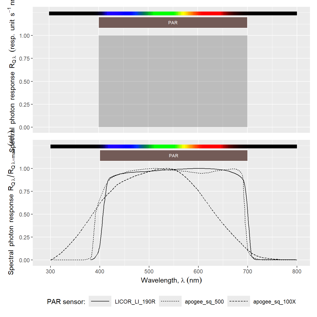
PAR sensors are in most cases based on silicon photodiodes filtered to change
the spectral response to better approximate that of the PAR BSWF. There is
considerable variation in how close this match is, although in no case the
deviation is as extreme as with photodiode-based pyranometers @fig-PAR-spct. Thus,
calibrations are dependent on the light spectrum to variable extents, and these
deviations should be taken into account when not using the sensors under the
light source they are calibrated to. In most cases, manufacturers calibrate PAR
sensors for sunlight.
```{r}
#| label: fig-PAR-spct
#| fig-asp: 1
#| fig-cap: Comparison of McCree's defintion of photosinthetically active radiation (PAR) to the spectral response of three PAR (=quantum) sensors. The three sensors are based on silicon photodiodes, with different filters. The Apogee SQ-100X is a low cost sensor while the other two are more expensive and using special optical filters. They are sold calibrated to give a reading approximating PAR when used in sunlight. The errors incurred when using such calibrations to measure light from other sources depends both on the sensor and on the light source.
autoplot(PAR(), range = c(300, 800), geom = "spct",
            unit.in = "photon", unit.out = "photon") /
  (autoplot(sensors.mspct[c("LICOR_LI_190R", "apogee_sq_500", "apogee_sq_100X")],
            idfactor = "PAR sensor:",
            w.band = PAR(),
            range = c(300, 800),
            annotations =c("-", "peaks"),
            unit.out = "photon") +
     theme(legend.position = "bottom")
  ) +
  plot_layout(axes = "collect")
```
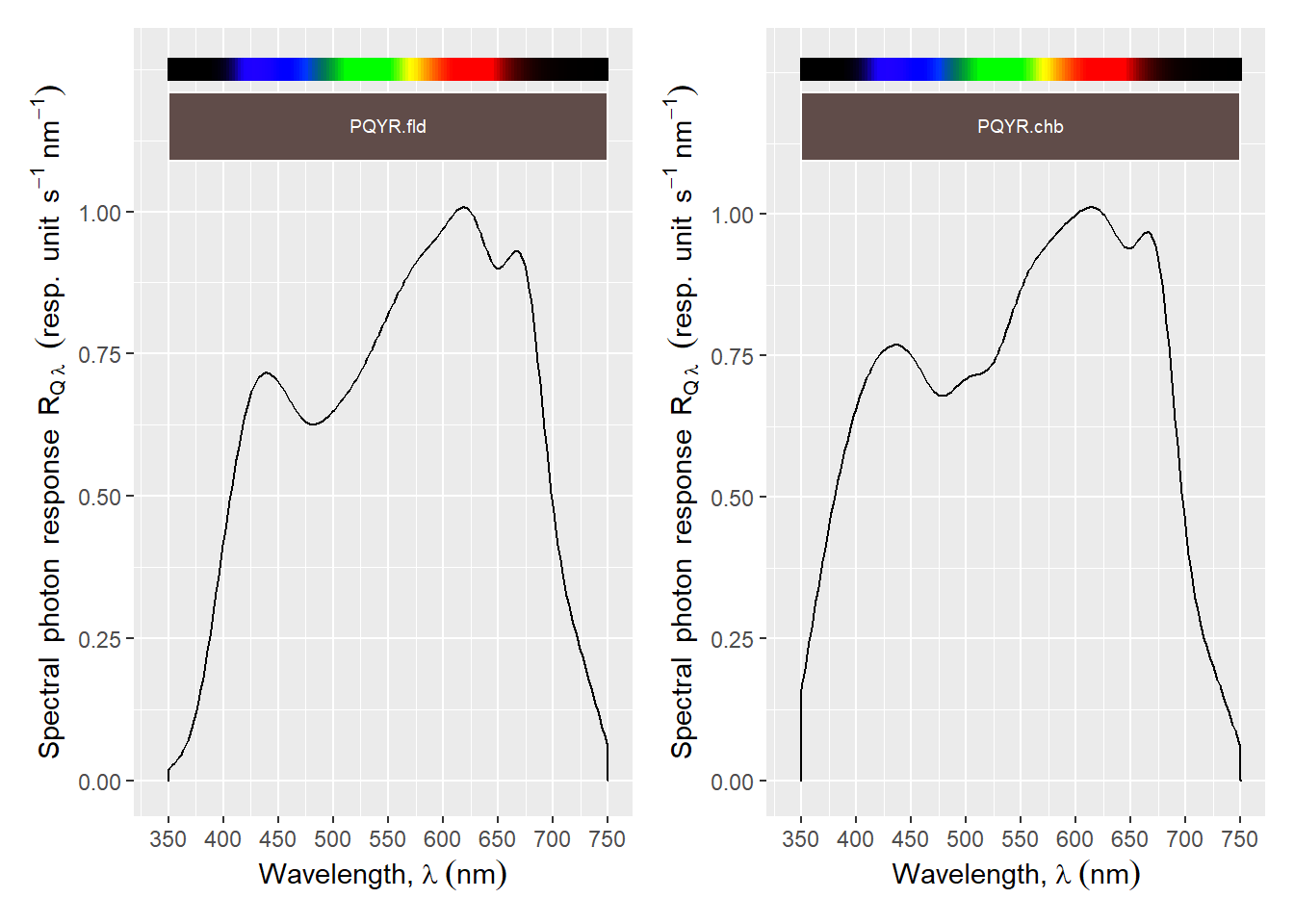
Some years after McCree proposed the use of PAR, another quantity was proposed
using the actual average of the action spectra measured by McCree as BSWF. It
was originally named Yield Photon Flux (originally YPF, here PQYR for
photosynthetic-quantum-yield weighted radiation). As McCree published two
different mean action spectra, one for field-grown crop plants and one for
growth-chamber-grown crop plants we end up with two new variations on
photosynthetically active radiation. This approach also extends the wavelength
range to that in the measured action spectra. No broadband sensors are available
for measuring PQYR and needs to be measured with a spectroradiometer or a PAR
sensor with a light-source specific calibration. @xxxx Bugbee et al tested the
difference....
```{r}
#| label: fig-PQYR-BSWF
#| fig-cap: The mean action spectra reported by McCree for leaves from field- and controlled-environment-grown crop plants and later used in the definition of YFD (PQYR eher). Normalised response as $\mathrm{CO_2}$ fixed per absorbed photon is plotted on the central wavelegth of 25 nm wide bands of illuminations used. The curves are interpolating natural spline.
autoplot(PAR("McCree.field.mean"),
         unit.in = "photon", unit.out = "photon") |
  autoplot(PAR("McCree.chamber.mean"),
           unit.in = "photon", unit.out = "photon")
```
It must be kept in mind that the original spectra were
measured under single colour light in bands 25 nm wide spaced by
25 to 30 nm. Differently to with McCree's definition, when calculating these
quantities the weights ($a_q(\lambda)$) applied are extracted directly from the
mean action spectrum curve, as for PAR, ignoring the difference between incident
and absorbed photons. The weights are different for energy and photon
spectral irradiance, corresponding to action spectra being expressed per unit
energy or per photon (or mole of photons).
$$Q_\mathrm{PQYR} = \int_{\mathrm{350\,nm}}^\mathrm{750\,nm} a_q(\lambda)\times
Q(\lambda)\ d \lambda$$
A more recent variation on PAR is extended PAR (ePAR) @ZhenXXX and justified in
that far-red photons can drive photosynthesis. Extended PAR is based on the same
simple photon-based BSWF as McCree's PAR but with the wavelength range extended
by 50 nm into the far red region, thus, based on a wavelength range of
$400\ldots 750$ nm.
$$Q_\mathrm{ePAR} = \int_\mathrm{400\,nm}^\mathrm{750\,nm} Q(\lambda)\ d \lambda$$
However, the role of far red light in photosynthesis is synergistic, known as
Emerson's effect. Far red light cannot drive photosynthesis on its own, but only
when shorter wavelengths are concurrently present with high enough photon
irradiance. Simple ePAR sensors like the SQ-610-SS from Apogee @fig-ePAR-spct
ignore this, and do give an ePAR reading higher than zero under pure far-red
radiation from LEDs and possibly too high readings under light from incandescent
lamps. When computing extended PAR from spectral data, the VIS light requirement
can be considered in the calculations and the value capped when needed to
account for the synergistic nature of the response to far red. We use xPAR to
describe the constrained version of ePAR. The factor 1.4 used in the equation
below is a coarse approximation.
$$Q_\mathrm{xPAR} = \mathrm{min}\left(1.4 \times \int_\mathrm{400\,nm}^\mathrm{700\,nm} Q(\lambda)\ d \lambda,\ \ \
\int_\mathrm{400\,nm}^\mathrm{750\,nm} Q(\lambda)\ d \lambda\right)$$
Apogee sells a two channel sensor, PAR + FR, (S2-141-SS) that makes this check possible.
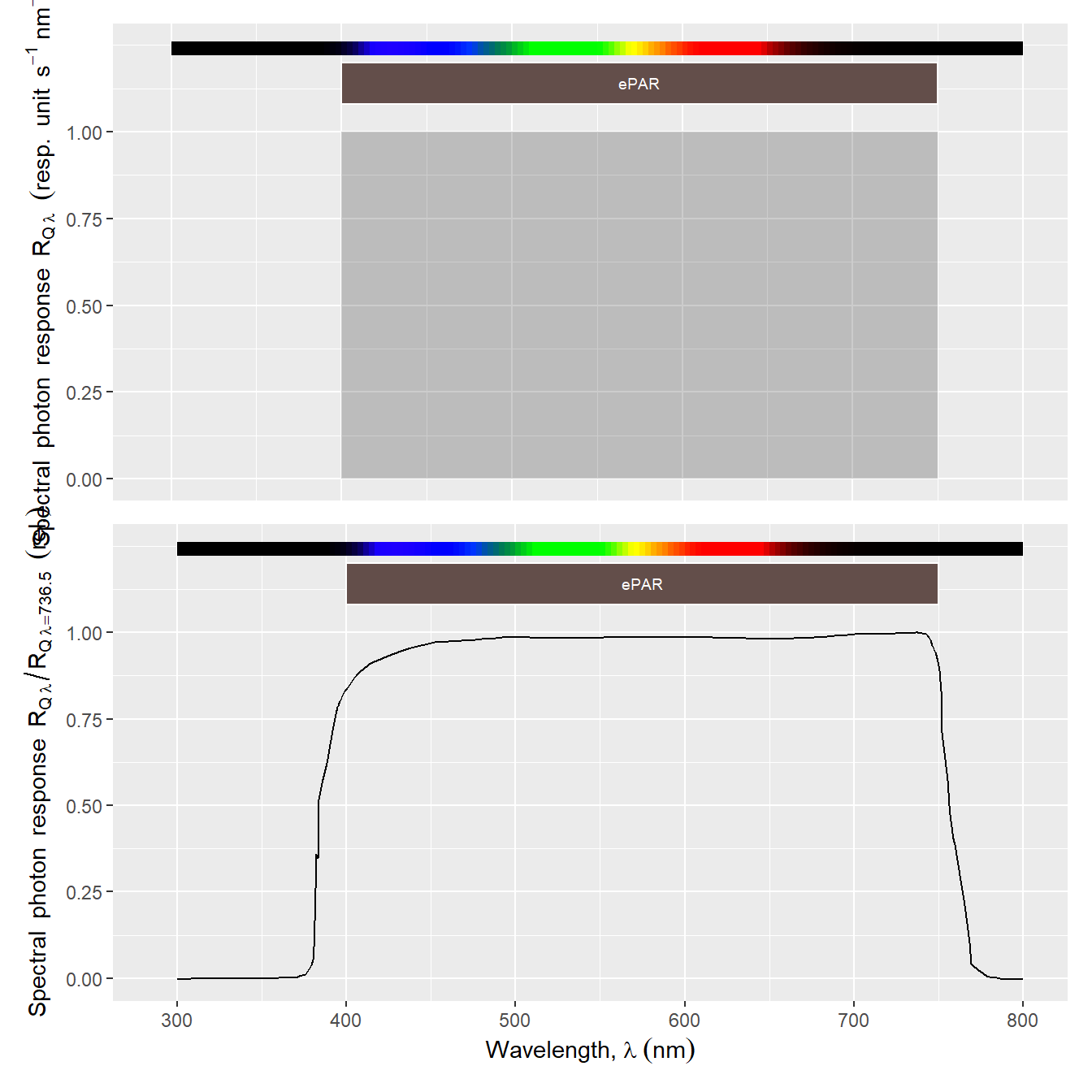
```{r}
#| label: fig-ePAR-spct
#| fig-asp: 1
#| fig-cap: Comparison of the definition of the ePAR to the spectral response of one single-channel ePAR sensor and a two-channel PAR + FR sensor. The two Apogee sensors are based on filterd silicon photodiodes, they are callibrated to give a reading approximating ePAR, PAR and FR in 700 to 750 nm when used in sunlight.
autoplot(PAR("ePAR"), range = c(300, 800), geom = "spct",
         unit.in = "photon", unit.out = "photon") /
  (autoplot(sensors.mspct[c("apogee_sq_610")],
            idfactor = "Pyranometer:",
            range = c(300, 800),
            annotations =c("-", "peaks", "summaries"),
            w.band = list(ePAR = PAR("ePAR")),
            unit.out = "photon") +
     theme(legend.position = "bottom")
  ) +
  plot_layout(axes = "collect")
```
Before the proposal of PAR by McCree two quantities based on similar wavelength
ranges were proposed as relevant to photosynthesis, but based on integrating
spectral energy irradiance. The @Gabrielsen1940 used the same wavelength
range as McCree's PAR ($400\ldots 700$ nm) while that proposed by Nichiporovich used a slightly
wider band of wavelengths one ($380\ldots 710$ nm).
With a spectroradiometer we can measure the spectral energy irradiance, and if
necessary convert it into spectral photon irradiance, and apply any of the
equations above to obtain measured values for the different quantities
described above. @tbl-PAR-ePAR-xPAR shows the results of applying this approach
to several different natural and artificial light sources. Most important is
that the differences among them depend on the spectrum of the light source.
```{r, echo = FALSE}
#| label: tbl-PAR-ePAR-xPAR
#| tbl-cap: Various photon irradiances ($Q_i$) used to quantify light useful for photosynthesis. PAR = McCree's PAR, ePAR = unconstrained extended PAR, xPAR = constrained extended PAR, FR = the far-red component of ePAR, PQYR = yield-spectrum weighted with .f for field and .c for chamber plants. For each light source, all values divided by $Q_\mathrm{PAR}$.
all_sources.mspct <-
source_mspct(list(sun = sun.spct,
sunlike.warm.led = leds.mspct$SeoulSemicon_S4SM_1564359736_0B500H3S_00001,
sunlike.cool.led = leds.mspct$SeoulSemicon_S4SM_1564509736_0B500H3S_00001,
blue.red.led = leds.mspct$Luminus_CXM_14_HS_12_36_AC30,
white.fr.led = leds.mspct$Ledguhon_10WBVGIR14G24_Y6C_T4,
cool.white.fluo = lamps.mspct$Osram.FT.L36W.865,
warm.white.fluo = lamps.mspct$Philips.CF.PLS.11W.927,
hps.discharge = lamps.mspct$Osram.HPS.Super.Vialox,
incandescent = lamps.mspct$Osram.Inc.20W,
hqit.multi.metal = lamps.mspct$Osram.MH.HQIT.400W,
Solray385.led = lamps.mspct$Valoya.LED.RX600HW.Solray385.grow.lamp,
AP67.led = lamps.mspct$Valoya.LED.B50.AP67.grow.lamp,
far.red.led = leds.mspct$Osram_GF_CSHPM2.24_2T4T_1))
all_sources.mspct <- setScaled(all_sources.mspct, scaled = FALSE)
all_sources.mspct <- msmsply(all_sources.mspct, setNormalised, norm = FALSE)
q_irrads.tb <- xPAR_irrad(all_sources.mspct, scale.factor = 1e6, w.band = list(PAR("McCree.field.mean"), PAR("McCree.chamber.mean"), PAR("Gaastra"), PAR("Nichiporovich")))
q_irrads.tb |>
mutate(Q_xPAR = round(Q_xPAR / Q_PAR, digits = 2),
Q_ePAR = round(Q_ePAR / Q_PAR, digits = 2),
Q_FR = round(Q_FR.700.750 / Q_PAR, digits = 2),
Q_FR.700.750 = NULL,
Q_PQYR.f = round(Q_PQYR.McCree.field.mean.550 / Q_PAR, digits = 2),
Q_PQYR.McCree.field.mean.550 = NULL,
Q_PQYR.c = round(Q_PQYR.McCree.chamber.mean.550 / Q_PAR, digits = 2),
Q_PQYR.McCree.chamber.mean.550 = NULL,
Q_Gaa. = round(Q_PAR.Gaastra / Q_PAR, digits = 2),
Q_PAR.Gaastra = NULL,
Q_Nich. = round(Q_PAR.Nichiporovich / Q_PAR, digits = 2),
Q_PAR.Nichiporovich = NULL,
Q_PAR = 1) |>
arrange(Q_FR) |>
kable()
```
Most PAR, or "quantum", sensors are based on silicon photodiodes, a filter to
constrain the range of wavelengths and a diffuser that provides an angular
response close to that proportional to the cosine of the angle of incidence of
light. No PAR sensor matches exactly the spectral response in the definition
of PAR or the cosine response. The best sensors provide a good approximation and
simpler (usually cheaper) sensors deviate more from PAR's definition and at low
angles of incidence.
In any light with a broad spectrum and no high peaks or deep valleys a good PAR
sensor will measure reasonably well PAR even if calibrated for sunlight. In
contrast, a simple PAR sensor calibrated in sunlight can be off by as much as
30% if used to measure light from an incandescent lamp. If used to measure a
light source with a narrow emission spectrum, such as a low pressure sodium lamp
or single colour LED, the error can be even larger. Such problems can be
resolved by use of light-source specific calibrations. Taken to the extreme,
if the light spectrum does not change, any sensor, even a bare photodiode that
responds to some of this light can be calibrated and used to measure PAR. Even
with the best PAR sensors, measurements of light from single-colour LEDs
emitting at some wavelengths, specially those near the boundaries near 400 and
700 nm, can be biased. When measuring single-colour LEDs using a broadband
sensor it is recommended to validate the sensor calibration against a
parallel measurement against a spectroradiometer. As photodiodes have an almost
perfectly linear response to irradiance, in most cases a single point calibration
is enough.
::: callout-warning
# Incident vs. absorbed photons
PAR photon irradiance quantifies the _incident_ flux of photons and is usually
measured on a horizontal plane. When studying the mechanism of photosynthesis,
in many cases it must be remembered that PAR irradiance can be very far from
being a measure of the flux of absorbed photons per unit leaf area. Leaves
differing in chlorophyll concentration per unit area, thickness, mesophyll cell
size and shapes, hairiness, cuticular waxes, and any other feature that modifies
their optical properties, can absorb different proportions of the PAR photons
incident on their surfaces. These differences as well as differences in
irradiance at the leaf plane due to differences in leaf display angle or in
light interception as a result of canopy structure must be taken into
consideration when interpreting responses to PAR. In fact, leaf absorptance is
dynamic as it depends on the accumulation movements of chloroplasts that have
time constants in the order of minutes.
:::
## Photon and energy ratios
One way of coarsely describing the shape of spectra is to express irradiance
in one region of the spectrum relative to that in a different region. In
photobiology photon ratios are the main interest, while in some applications
energy ratios or photon to energy ratios are relevant.
We can, for example, compute the red to far-red (R:FR) photon ratio, relevant to
responses mediated by the photoreceptor phytochromw, as the ratio between two
photon irradiances.
$$Q_\mathrm{red}:Q_\mathrm{far\ red} = \frac{\int_{\lambda = 650\,\mathrm{nm}}^{\lambda = 670\,\mathrm{nm}} Q(\lambda) \,d\lambda}{\int_{\lambda = 725\,\mathrm{nm}}^{\lambda = 745\,\mathrm{nm}} Q(\lambda) \,d\lambda}$$
where $\lambda$ is wavelength, $Q$ photon (= quantum) is irradiance and
$Q(\lambda)$ spectral photon irradiance. In this example using the most
frequently used 20-nm-wide wavelength bands centred at
$\lambda = 660\,\mathrm{nm}$ for red light and at $\lambda = 735\,\mathrm{nm}$
for far red light (\cite{Smith1981}). (It is possible to use in place of
irradiances, time integrated quantities such as fluence, as long as the time
and spatial bases of expression used for the numerator and denominator are
the same).
Two main kinds of photon ratios are in use in plant photobiology. Ratios like
the red to far-red (R:FR) photon ratio computed above in which the photon
irradiances in the numerator and denominator are for non-overlapping wavelength
regions, and ratios such as the ultraviolet-B to total ultraviolet (UVB:UV)
photon ratio where the wavelength band used for the numerator is a spectral
region within that used for the denominator. Ratios between non-overlapping
regions can _in principle_ take any unit-less numeric value in $-\inf\ldots\inf$
while ratios in which the numerator wavelength range is nested in the wavelength
range of the denominator can take _at most_ numeric values in $0\ldots1$.
```{r, eval=TRUE, include=FALSE}
# pre-compute for in-line printing below
qq <-
round(
as.numeric(
photobiology::q_ratio(photobiology::sun.spct,
UVB(), PAR())) * 1000,
digits = 1)
ee <-
round(
as.numeric(photobiology::e_ratio(photobiology::sun.spct,
UVB(), PAR())) * 1000,
digits = 1)
```
It is also possible, although less common, to define ratios based on energy. It
important to keep in mind that a photo ratio and an energy ratio based on the
same wavelength ranges will differ. As seen for the conversion between photon
and energy irradiances in section XXXXX, the conversion is possible only if the
spectral irradiance is know as it is a function of wavelength. For example,
based on a sunlight spectrum for the mid-morning in the Spring in Helsinki the
UV-B:PAR photon ratio of `{r} qq` ‰ corresponds to an UV-B:PAR energy
ratio of `{r} ee` ‰.
Finally, photon to energy ratios are also in use. In this case the range of
wavelengths used for the numerator and denominator are the same but the
irradiance in the numerator is expressed as a flux of photons and that in the
denominator as a flux of energy. As the energy per photon depends on wavelength,
the photon to energy ratio increases with increasing wavelength.
Although less accurate than a spectrum with higher wavelength resolution, ratios
provide summaries that are easier to interpret and analyse, and in many cases
also easier to measure. One should, however, be careful with the interpretation
of ratios as they are coarse summaries. Ratios discard important information
about the shape of the spectrum as a whole and consequently the relationship
between photon ratios and biological responses frequently is interpretable only
when regions of the spectrum are reasonably close to those in the daylight
spectrum.
It is very important to conduct experiments under realistic
environmental conditions, i.e., conditions relevant to the aims of a study. For
studies to be relevant to plants growing outdoors, these conditions include
the daylight spectrum, while in contrast, for controlled environment farming,
a good match to the spectrum of the artificial light used.
For the assessment and control of experimental conditions, it is
helpful---besides using biologically effective irradiances and exposures---to
calculate photon ratios to assess the similarity or not of illumination. Photon
ratios inform succinctly about differences among experimental conditions or
between experimental conditions and
As
for example shown in section
[8.2.7](#sec:simulators){reference-type="ref"
reference="sec:simulators"} on page and in table
[\[tab:typical:irrad:values\]](#tab:typical:irrad:values){reference-type="ref"
reference="tab:typical:irrad:values"} on page. For the calculation of
these ratios, it is essential to use the same quantity of
radiation or the same weighting procedure, i.e. energetic
units or photon units for the ratios being compared.
### A practical example
The importance of indicating the type of sensor and its orientation is
exemplified by the changing ratio of fluence rate to irradiance
throughout a day (Figure
[\[fig:fluence:rate:irradiance\]](#fig:fluence:rate:irradiance){reference-type="ref"
reference="fig:fluence:rate:irradiance"}). At noon, when the sun is high
in the sky the ratio is at its minimum. Even then the ratio remains
larger than one because, other than at the equator, the midday sun never
reaches the zenith and because the sensor will also always receive
diffuse radiation from the whole sky. We can say that when measuring
solar radiation the fluence rate will always be numerically larger than
the irradiance. Towards both ends of the day the ratio reaches its
maximum value because irradiance is being measured on a horizontal plane
but the sun is near the horizon. During twilight, particles in the
atmosphere will make the distribution of solar radiation more even,
allowing a relatively large area of the sky to remain bright, and the
ratio decreases again.
::: figure*
{width="0.8\\myfigwidth"}
:::
### Measuring fluence rate and radiance
Spherical sensors, as needed for measuring fluence rate, also called
scalar irradiance, are not common. LI-COR (Lincoln, NE, USA) sells a
spherical quantum sensor (LI-193) that can be submerged, and
Biospherical Instruments Inc. (San Diego, CA, USA) makes both PAR-
(e.g. QSL-2100 and QSL-2200, terrestrial; QSP series with models that
can be submerged to thousands of metres) and also narrowband spherical
sensors for measuring UV- and visible radiation fluence rate.
Biospherical Instruments Inc. also makes radiance sensors with input
optics that have a very narrow acceptance angle. Figure
[\[fig:AMOUR:entrance:optics\]](#fig:AMOUR:entrance:optics){reference-type="ref"
reference="fig:AMOUR:entrance:optics"} shows the different entrance
optics available for one series of sensors from Biospherical
Instruments. Most broadband UV sensors and entrance optics for
spectroradiometers follow a cosine response. @Bjorn1995 describes a
method for estimating fluence rate from three or six irradiance
measurements at a series of specific angles.
::: figure*
{width="0.8\\myfigwidth"}
:::
### Sensor output
Radiometer sensors can have either analog or digital outputs. Some
sensors with an analogue output have an amplifier next to the detector,
others do not. Sensors with an analog output are usually connected to a
voltmeter or a datalogger. Some digital sensors are really complete
radiometers with a digital output. Examples of radiometers with digital
outputs, are shown in Figure
[\[fig:AMOUR\]](#fig:AMOUR){reference-type="ref" reference="fig:AMOUR"}.
RS-232 and USB are digital interfaces frequently used to attach these
sensors to personal computers[^19].
::: figure*
{width="0.8\\myfigwidth"}
:::
### Calibration
To calibrate radiation sensors the relationship must be determined
between the electrical signal produced by a sensor and the amount of
radiation impinging on that sensor. The physical value of irradiance, ,
of the incoming radiation in energy units, is obtained by "comparison"
of a measurement $X$ with that of a calibrated radiation source
$X_\mathrm{lamp}$,
$$\irr = \irr[lamp] \cdot \frac{X\cdot a}{X_\mathrm{lamp}}$$ where
$\irr[lamp]$ is the calibration file of the lamp provided by the
calibration survey. The factor $a$ accounts for any difference in the
lamp to sensor distance between the survey's calibration and your own
measurement of the lamp. In most modern instruments this "comparison" is
implicitly done by the software in the instrument itself, or the
computer it is attached to, by multiplying the electrical signal from
the detector with a calibration constant. If this is not the case, it is
necessary to correct all raw measurements, here $X$ and
$X_\mathrm{lamp}$, before making any further calculations, for example,
by subtracting the measurement of dark current (the sensor reading in
the dark).
Although photons can be counted using a photomultiplier and appropriate
electronics, this approach does not provide an absolute measurement.
Some photons are always missed and false counts are included due to
thermal excitation. Therefore, absolute calibration of radiation meters
can only be provided in energetic terms. For this purpose so-called
"blackbody radiators" of known temperature are used, since they depend
only on temperature for the total radiation as well as its spectral
distribution. Blackbody radiators used for the calibration of lamps, are
then available for purchase by scientists for use as secondary
standards.
In the case of broadband sensors used to measure biologically-effective
irradiances or selected bands of the spectrum, the calibration is
usually carried out by comparison to readings from a calibrated
spectroradiometer under a radiation source with a spectrum as similar as
possible to the one which will be measured with the broadband sensor
(e.g. sunlight). To calibrate spectroradiometers, in addition to a
spectral-irradiance calibration against one or more lamps (with a
continuous spectrum, such as an incandescent lamp), it is necessary to
do a wavelength calibration against the sun or a lamp (with a an
emission spectrum with discrete, narrow and stable peaks, such as a low
pressure mercury lamp).
### Further reading {#further-reading}
@Bjorn1996b treat the same subjects as this section, but in more depth.
Also the book edited by @Bjorn2007 is a good source of basic information
about radiation and photobiology.
## Actinometry
Actinometers are chemical systems for the measurement of light and
ultraviolet radiation. They do not need to be calibrated by the user,
and thus do not require the purchase of an expensive standard lamp with
an expensive power supply. Standardization has usually been taken care
of by those who have designed the actinometer. Another advantage is that
their geometry can more easily be adjusted to the measurement problem.
The shape of a liquid actinometer can be made to correspond to the
overall shape of the irradiated object under study.
In many cases, it is of interest to study a suspension or solution that
can be put in an ordinary cuvette for spectrophotometry or fluorimetry,
and the actinometer solution can be put into a similar cuvette. A large
number of actinometers have been devised. @Kuhn1989 lists, briefly
describes and gives references for 67 different systems of which they
recommend five. In general, actinometers are sensitive to short-wave
radiation ($<$`<!-- -->`{=html}500 nm) and insensitive to long-wave
radiation ($>$`<!-- -->`{=html}500 nm). Insensitivity to long-wave
radiation can be both a drawback and an advantage, but by choosing the
best actinometer for a particular purpose we can avoid their
disadvantages. One advantage of using an actinometer insensitive to long
wave radiation is that we can use it for UV work under illumination
visible to the human eye, without disturbing the measurement. Here we
shall concentrate on the most popular actinometer for ultraviolet
radiation---the potassium ferrioxalate or potassium iron(III) oxalate
actinometer. In addition to using it directly in some experiments, we
can use it for checking the calibration of other instruments, such as
spectroradiometers.
The description below is sufficient for a researcher starting to work in
the field. For more detailed information one should consult @Parker1953
[@Hatchard1956; @Lee1964; @Goldstein2008]. Complete recipes have also
been published, e.g., @Seliger1965 [@Jagger1967]. In the ferrioxalate
actinometer the following photochemical reaction is exploited:
::: centering
$\frac{1}{2}$ (COO)$_2^{2-}$ + Fe$^{3+}$ + photon $\rightarrow$ CO$_2$ +
Fe$^{2+}$\
or\
Oxalate ion + Fe(III) ion + radiation $\rightarrow$ carbon dioxide +
Fe(II) ion\
:::
The quantum yield for this reaction (i.e., the number of iron ions
reduced per photon absorbed) is slightly wavelength dependent but close
to 1.26 in the spectral region, 250--500 nm, where the ferrioxalate
actinometer is used. Usually a 1-cm layer of 0.006 M ferrioxalate
solution is used. Quantum yield and the fraction of radiation
(perpendicular to the 1 cm layer) absorbed are shown in Table
[\[tab:ferrioxlate\]](#tab:ferrioxlate){reference-type="ref"
reference="tab:ferrioxlate"}.
As seen from Table
[\[tab:actinometer\]](#tab:actinometer){reference-type="ref"
reference="tab:actinometer"} the sensitivity of this actinometer (column
to the right) is constant throughout most of the UV range, which makes
it very convenient for our work.
The amount of Fe(II) formed can be measured spectrophotometrically after
the addition of phenanthroline, which gives a strongly absorbing yellow
complex with Fe(II) ions.
The ferrioxalate (actually potassium ferrioxalate) for the actinometer
is prepared by mixing 3 volumes of 1.5 M potassium oxalate (COOK$_{2}$)
with 1 volume of 1.5 M FeCl$_3$ and stirring vigorously. This step and
all the following procedures involving ferrioxalate should be carried
out under red light (red fluorescent tubes or LEDs). The precipitated
should be dissolved in a minimal amount of hot water and the solution
allowed to cool for crystallization (this crystallization should be
repeated twice more). Potassium ferrioxalate can also be purchased
ready-made, but the price difference encourages self-fabrication. The
following is a recipe for the three solutions required to carry out
actinometry [see @Goldstein2008 for a different procedure and other
quantum yields]:
**Solution A:** Dissolve 2.947 g of the purified and dried K$_3$Fe(III)
oxalate in 800 ml distilled water, add 100 ml 0.5 M sulfuric acid, and
dilute the solution to 1000 ml. This gives 0.006 M actinometer solution,
which is suitable for measurement of ultraviolet radiation.
**Solution B:** The phenanthroline solution to be used for developing
the colour with Fe(II) ions should be 0.1% w/v 1:10 phenanthroline
monohydrate in distilled water.
**Solution C:** Prepare an acetate buffer by mixing 600 ml of 0.5 M
sodium acetate with 360 ml of 0.5 M H$_2$SO$_4$.
Solution A is irradiated with the radiation to be measured. The
geometries of both the container and of the radiation are important and
must be taken into account when evaluating the result. The simplest case
is when the radiation is [collimated]{acronym-label="collimated"
acronym-form="singular+short"}, the container a flat spectrophotometer
cuvette, the radiation strikes one face of the cuvette perpendicularly,
and no radiation is transmitted. Even in this case one has to
distinguish between whether the cuvette or the beam has the greater
cross section, and correct for reflection in the cuvette surfaces. The
irradiation time should be adjusted so that no more than 20% of the iron
is reduced (this corresponds to an
[absorbance]{acronym-label="absorbance" acronym-form="singular+short"}
of about 0.66). In the following we shall assume that we use an ordinary
fused-silica or quartz spectrophotometer cuvette with 10 mm inner
thickness and containing 3 ml actinometer solution.
After the irradiation and mixing of the actinometer solution, 2 ml of
the irradiated solution is mixed with 2 ml of solution B and 1 ml of
solution C, and then diluted to 20 ml with distilled water. After 30
minutes the absorbance at 510 nm is measured against a blank made up in
the same way with unirradiated solution A. An absorbance of 0.5
corresponds to 0.905 $\mymu$mol Fe$^{2+}$. It is a good idea to check
this relationship with known amounts of FeSO$_4$ if you have not
previously checked your spectrophotometer for accuracy and linearity.
You should not use any absorbance above 0.65.
Example of calculation: 3 ml of 0.006 M actinometer solution are
irradiated by parallel rays of 300 nm UV-B impinging at right angles to
one surface (and not able to enter any other surface). The radiation
cross section intercepted by the solution is 2 cm$^2$. Five minutes of
irradiation produces an absorbance of 0.6. This corresponds to
$0.6 \cdot 0.905/0.5$ $\mymu$mol = 1.086 $\mymu$mol Fe$^{2+}$, but since
we have taken 2 out of the 3 ml actinometer solution for analysis,
multiply by 3/2 to get the total amount of Fe$^{2+}$ formed. Throughout
the UV-B region the quantum yield is 1.26, so this corresponds to
absorption of $3 \cdot 1.086/2/1.26$ $\mymu$mol photons. Reflection from
the surface is estimated to be 7% (by application of Snell's law, or law
of refraction, giving the angle of refraction for an angle of incidence
at the boundary of two media like water and glass). None of the
radiation penetrates the solution to the rear surface, since the
solution thickness is 1 cm. Therefore the incident radiation is
$3 \cdot 1.086/(1.26 \cdot 0.93 \cdot 2)$ $\mymu$mol = 1.390 $\mymu$mol
radiation incident on 2 cm$^2$ in 5 minutes, and the photon irradiance
(quantum flux density, in this case equal to the photon fluence rate,
since the rays are parallel and at right angles to the surface) is
1.390/(2$\cdot$`<!-- -->`{=html}5) $\mymu$mol/cm$^2$/min = 0.1390
$\mymu$mol/cm$^2$/min = $10000 \cdot 0.1390/60$ $\mymu$mol/m$^2$/s =
23.2 $\mymu$mol/m$^2$/s.
@Kirk1983 point out errors that might arise if a more concentrated
actinometer solution is used, in order to absorb more light at long
wavelengths, and how these errors can be minimized. If an actinometer
much more concentrated than 0.006 M is used, the quantum yield is lower,
and we do not recommend this for UV research. @Goldstein2008, using
0.06 M actinometer solution, find almost the same quantum yield (1.24)
from 250 to 365 nm, but much higher (1.47) from 205 to 240 nm; the
latter in marked contrast to the values of @Fernandez1979 in the table
above, so measurements below 250 nm should be regarded with caution.
@Bowman1976 warn against exposure of the phenanthroline solution to UV,
and even against the fluorescent room lighting.
Chemical or biological systems (mostly in a solid state) for recording
solar radiation and particularly radiation, are widely employed for
estimating the exposure of people, leaves in a plant canopy, and other
objects which for various reasons are not easily amenable to
measurements with electronic devices. These chemical devices are
generally referred to as dosimeters rather than actinometers, even if
there is no defined delimitation between these categories. As the
construction, calibration, and use of chemical and other dosimeters have
been the subject of frequent reviewing
[@Berces1999; @Horneck1996; @Marijnissen1987], we shall not dwell on
them here, only stress that their radiation sensitive components can be
either chemical substances (natural such as DNA or provitamin D, or
artificial) or living cells (e.g., various spores and bacteria).
## Dosimeters
Broadband dosimeters have been developed to quantify exposure to UV
radiation based either upon the photochemical degradation of chemical
compounds and plastic films or using biological techniques involving
damage to DNA. The range of experimental methods has been described by
@Dunne1999 and @Parisi2010a. The most practical and effective dosimeters
for plant studies include the use of plastic films of polysulphone (PS)
and poly 2,6-dimethyl-1,4-phenylene oxide (polyphenylene oxide or PPO)
[see @Geiss2003; @Parisi2010b] and the determination of spore viability
after UV exposure [see e.g.
@Quintern1992; @Quintern1994; @Quintern1997; @Furusawa1998].
A commercially available UV-dosimetry system '*Viospor*' (Biosense,
Germany) uses the DNA molecules of microbial spores immobilised in a
film mounted in a protective casing with a cosine corrected filter
system to provide a measurement of biologically-weighted UV exposure
(Figure
[\[fig:UV:dosimeters:VS\]](#fig:UV:dosimeters:VS){reference-type="ref"
reference="fig:UV:dosimeters:VS"}). *Viospor* sensors are available as
two types: *Viospor* blue-line types I-IV which provide estimates of the
CIE erythemal exposure (as MED, J m-2, and SED) at a range of exposure
levels from seconds to several days, and *Viospor* red-line which use
the DNA damage action spectrum [@Setlow1974] to estimate the DNA
damaging capacity of UV-B and UV-C radiation and the efficiency of UV-C
germicidal lamps. After exposure, films are incubated in bacterial
growth medium to stimulate spore germination and the production of
proteins that are stained for densitometric quantification. Exposed
dosimeters are returned to the supplier for analysis (***BioSense***,
Dr. Hans Holtschmidt, Laboratory for Biosensory Systems, Postfach 5161,
D-53318 Bornheim, Germany. phone: +49-228-653809, fax: +49-228-653809,
[mailto:mail@biosense.de](mailto:mail@biosense.de){.uri}, internet:
<http://www.biosense.de>).
::: figure*
{height="3.7cm"} {height="3.7cm"}
:::
Small dosimeters have also been constructed from 30--45 film of the
thermoplastic polysulphone and can be used to determine exposure by
measuring the increase in [absorbance]{acronym-label="absorbance"
acronym-form="singular+short"} at 330 nm [@Geiss2003; @Parisi2010a]
ideally using an integrating sphere to minimise the effects of
scattering (Figure
[\[fig:UV:dosimeters:PS\]](#fig:UV:dosimeters:PS){reference-type="ref"
reference="fig:UV:dosimeters:PS"}). Dosimeters can be calibrated in
sunlight by comparison with erythemally-calibrated broadband radiometers
or against lamp sources using a double monochromator spectroradiometer.
Ideally, the calibration should be determined under field conditions
appropriate for plant studies and if calibrated outside in sunlight the
calibration is only accurate under the prevailing atmospheric ozone
column as this modifies the UV spectrum. An erythemal dose can be
calculated from 40 polysulphone film using a relationship of the form
[see @Geiss2003]:
$$\mathrm{Radiation\ amount}\ (\Unit{J\,m^{-2}}) = 8025\, (\Delta \mathrm{A}_{330})^2 + 1980.8\, \Delta \mathrm{A}_{330}$$
where is the absorbance at 330 nm before exposure (which should be
between 0.105 and 0.133) minus the absorbance at 330 nm after exposure
plus a further 24 h in the dark. The film may also be calibrated against
other action spectra.
Accuracy of polysulphone dosimetry has been reported to be
$\pm$`<!-- -->`{=html}10% if is $<$`<!-- -->`{=html}0.3 but decreases to
$\pm$`<!-- -->`{=html}30% for up to 0.4 [@Diffey1987]. Greater
variability in occurs with increasing duration of exposure and
dosimeters saturate at sub-tropical sites in less than one day. However,
they have also been modified with a filter to provide an extended
dynamic range of exposure (over 3 to 6 days) without the need to replace
the dosimeter due to saturation [@Parisi2004a]. Polysulphone dosimeters
have been combined with a PAR dosimeter to investigate the visible and
UV radiation environment of plants [@Parisi1998; @Parisi2003] and
miniature versions have also been developed:
$1.5~\Unit{cm} \times 1.0~\Unit{cm}$ with an exposure of a 6 mm disc of
polysulphone [@Parisi2010a].
::: figure*
{width="0.4\\myfigwidth"} {width="0.4\\myfigwidth"}
:::
For longer exposure periods, dosimeters using an alternative plastic
film, PPO, have been found more suitable as they saturate at
sub-tropical locations after 5--10 days. The change in absorbance of PPO
is quantified at 320 nm and it has been successfully calibrated to
erythemal exposures [@Lester2003] and by using a mylar (polyester)
filter for estimation of UV-A exposures [@Turnbull2008]. Both PS and PPO
dosimeters have been investigated for underwater use where PPO has been
considered viable when calibrated under water (but not using a
calibration in air) and under the relevant ozone column conditions of
the study [@Schouten2007; @Schouten2008]. The duration of use of PPO
dosimeters in air at sub-tropical locations has been extended from 5 to
10 days by the use of neutral density filters
[@Parisi2010b; @Schouten2010].
The use of properly calibrated UV dosimeters can be particularly
valuable in plant studies when long-term use of spectroradiometers and
broadband radiometers is restricted by availability of electrical
supplies or by physical constraints.
## Thermopiles
Most thermopiles have a flat response to (energy) irradiance across a
wide range wavelengths. They are arrays of thermocouples formed between
two different metal alloys. In a thermopile some couples are painted
white and some black (or some other arrangement is used to generate a
temperature difference dependent on absorbed energy), and the difference
in temperature induced by the absorption of radiation by the black
regions generates an electrical signal. A single thermocouple produces a
very small signal, but connecting them in series generates a large
signal that is easier to measure. Thermopiles can be either small for
use in the laboratory or larger, and protected by a quartz dome for use
in the field. Thermopile pyranometers are used to measure solar
radiation in the range 285 to 2800 nm. Examples of such instruments are
the pyranometers in the CMP series from Kipp & Zonen. Thermopile
pyranometers are standard instruments in weather stations. Thermopiles
can be also used to measure the (energy) irradiance of monochromatic
radiation, including radiation, if the dome or 'window' is made from an
transparent material.
## Broadband instruments
UV broadband radiometers integrate over either the UV-A or UV-B band or
both, which encompasses the entire UV region of daylight. The names
broadband and narrowband refer to the width of the 'window' or range of
wavelengths to which a sensor responds. The term full-width half-maximum
(FWHM) is used to measure this, it means the width of the peak in units
of wavelength, measured at half the maximum height of the peak along the
$y$-axis (with the output of the sensor on the $y$-axis plotted on a
linear scale). A narrow band-pass can have a 10 nm or 20 nm FWHM while a
wide one can have an 80 nm FWHM for instruments measuring a combination
of UV-A and UV-B radiation.
Their low cost, fast response (typically milliseconds to seconds),
stability and low maintenance requirements make them suitable for
continuous monitoring applications. The most common spectral response is
one that follows the erythemal action spectrum defined by the Commission
Internationale de l'Eclairage, or CIE, [@McKinlay1987; @Webb2011], which
describes the response of the human skin to UV radiation (Figure
[\[fig:action:spectra\]](#fig:action:spectra){reference-type="ref"
reference="fig:action:spectra"}, on page ).
However, erythemally effective can be derived from most UV measuring
instruments if the radiation spectrum is known and fairly stable in time
such as when measuring sunlight. Hence, in meteorology the UV index is
taken as a common factor that should be obtained from the data at every
measuring site. Vice versa, using a correction factor to the
instrument's output, actual erythemal irradiance in effective can be
calculated. Data from UV broadband instruments are part of a worldwide
UV database that is located in the World Ozone and Ultraviolet Radiation
Data Centre (WOUDC) as a part the Global Atmosphere Watch (GAW)
programme of the World Meteorological Organization (WMO).
As the spectral response of broadband radiometers only approximately
follow the needed for the desired response, their use for measuring
different radiation sources requires source-specific calibration. The
readings of broadband radiometers calibrated for sunlight should not be
used to assess doses from lamps without using correction factors
obtained by calibration. For measuring lamps and LEDs the use of a
spectroradiometer is strongly recommended.
### Principle of operation {#sec:broadband:principles:operation}
The basic design of broadband instruments has not changed significantly
since the introduction of the first erythemally weighted solar
radiometer, the Robertson-Berger meter [@Robertson1972; @Berger1976].
When direct and scattered solar radiation is transmitted through the
transmitting quartz dome, the most common way to obtain an erythemal
weighting is to filter out nearly all visible light using -transmitting
black-glass blocking filters. The remaining radiation then strikes a
sensitive fluorescent phosphor to convert UV-B light to visible light,
i.e. green light emitted by the phosphor. This light is filtered again
using coloured glass to remove any non-green visible light before
impinging on a gallium arsenic or a gallium arsenic phosphorus
photodiode used as detector.
::: figure*
{width="0.55\\myfigwidth"}
:::
A thermally stable amplifier converts the diode's output current to a
voltage. It drives a line amplifier that provides a low impedance 0 to
+4 V DC output signal. Phosphor efficiency decreases by approximately
0.5% K$^{-1}$ and its wavelength response curve is shifted by
approximately 1 nm towards the red every 10 K. This latter effect is
particularly important because of the slope of the solar radiation curve
at these wavelengths. The glass filters, phosphor and photodiode are
held at 25 to 50, depending on the manufacturer, to ensure that the
output signal is not sensitive to changes in ambient temperature.
Temperature stabilization is usually achieved by an internal thermistor
that permits independent monitoring of the sensor's temperature (Figure
[\[fig:Yankee\]](#fig:Yankee){reference-type="ref"
reference="fig:Yankee"}). The analogue electrical signal produced by the
broadband UV instrument is converted into digital format for electronic
logging. The sampling frequency is usually between once per second (1
Hz) and once per minute. If the complete data set is not stored then
data are saved as averages over periods ranging from 10 minutes to not
more than one hour. Sometimes, the variation around the mean is also
recorded for each averaging period. This indicates the constancy of the
conditions during the averaging period (e.g. sun screening by rapidly
changing cloud cover: broken clouds or clear sky or constant
cloudiness). The raw signal must be converted into units of erythemal
irradiance () using a calibration factor, plus several corrections.
These corrections require additional data: solar zenith angle () and
ozone column depth at the time of measurement.
Erythemal effective irradiance () is calculated [@Webb2006]:
$$\irr[CIE] = (\voltage - \voltage[d]) \cdot k \cdot f(\SZA, \TOthree) \cdot f(\temperature) \cdot \Coscor$$
Where: $\voltage$ is the measured electrical signal from the radiometer,
$\voltage[d]$ is the electrical offset for dark conditions, $k$ is the
calibration coefficient, a constant value determined for specific
conditions, e.g. at of 40and a total ozone column of 300 DU[^20].
$f(\SZA, \TOthree)$ is a function of the solar zenith angle () and the
total column of ozone (), i.e. the function can be expressed as a
calibration matrix (or look up table) and is derived as part of the
calibration procedure. It is normalized at a solar zenith angle of 40and
a total ozone column of 300 DU. For solar zenith angles less than 40,
$f(\SZA, \TOthree)$ is often nearly unity. $f(\temperature)$ is the
temperature correction function. It is recommended that the instrument
is temperature stabilized. If this is not applicable then a correction
should be applied, which is complex and not always successful. $\Coscor$
is the cosine correction function (if necessary, otherwise =1).
The quality of the broadband instrument depends on the quality of the
protective quartz dome, the cosine response, the temperature stability,
and the ability of the manufacturer to match the erythemal curve with a
combination of glass and diode characteristics. Instrument temperature
stability is crucial, with respect to both the electronics and the
response of the phosphor to the incident UV radiation.
More recently, broadband instruments are using thin film metal
interference filter technology and specially developed silicon
photodiodes to measure UV erythemal irradiance. This overcomes many
problems connected with the phosphor technology, but on the other hand
they have difficulties related to very low photodiode signal levels and
filter stability. Silicon carbide () photodiodes have good sensitivity
to radiation and are intrinsically blind to visible radiation.
Other broadband instruments use one of these measurement technologies to
measure other regions of the spectrum by using either a combination of
glass filters or interference filters. Some manufacturers of these
instruments provide simple algorithms to approximate erythemal dosage
from the unweighted measurements [@WMO2008].
The maintenance of broadband instruments consists of ensuring that the
domes are cleaned, the instrument is level, the desiccant (if provided)
is active, and the heating/cooling system is working correctly, if so
equipped.
### Some commonly used terrestrial instruments {#sec:broadband:instruments}
The most common outdoor broadband radiometers are: SL 501 from Solar
Light, Inc. (Glenside, PA, USA), YES UVB-1 from Yankee Environmental
Systems, Inc. (Turners Falls, MA, USA), UVS-E-T (erythemal), UVS-A-T
(UV-A) and UVS-B-T (UV-B) from Kipp & Zonen (Delft, The Netherlands)
(Figure
[\[fig:UV:pyranometers\]](#fig:UV:pyranometers){reference-type="ref"
reference="fig:UV:pyranometers"}). The principle of operation of these
meters is basically the same as described in section
[9.5.1](#sec:broadband:principles:operation){reference-type="ref"
reference="sec:broadband:principles:operation"}. Unlike the other
meters, the Scintec UV-S-290-T uses a Teflon diffuser under the quartz
dome in front of the filters. These three instruments are temperature
stabilized by means of heating elements and temperature sensors. Solar
light also sells non-stabilized instruments like the PMA2101 (digital)
and PMA1101 (analog), which contain a temperature sensor whose output
can be used to correct in silico for the temperature dependency of the
UV-B readings.
::: figure*
{width="0.3\\myfigwidth"} {width="0.3\\myfigwidth"} {width="0.3\\myfigwidth"}
:::
Broadband sensors based on special silicon photodiodes are also
available, which, are more stable with respect to variation in
temperature than those based on phosphors. Delta-Ohm (Padova, Italy),
Delta-T Devices (Cambridge, UK) and Sky instruments (Llandrindod Wells,
UK) make sensors based on this principle. Examples are the SKU 420, SKU
430, and SKU 440 (UV-A, UV-B, and erythemal, respectively) from Sky
Instruments, LP UVA 01/03 and LP UVB 01/03 from Delta-Ohm, and UV3pB-05
and UV3pA-05 from Delta-T devices (Figure
[\[fig:UV:diode:sensors\]](#fig:UV:diode:sensors){reference-type="ref"
reference="fig:UV:diode:sensors"}). All of them are UV radiometers with
no temperature stabilization or in-built temperature sensors.
International Light Technologies (Peabody, USA) makes a wide array of
meters and sensors for measuring radiation. Vital Technologies used to
make good UV sensors which were popular some years ago, but the company
is no longer in business. Most of these sensors have built-in
preamplifiers.
::: figure*
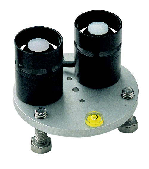{height="5cm"} 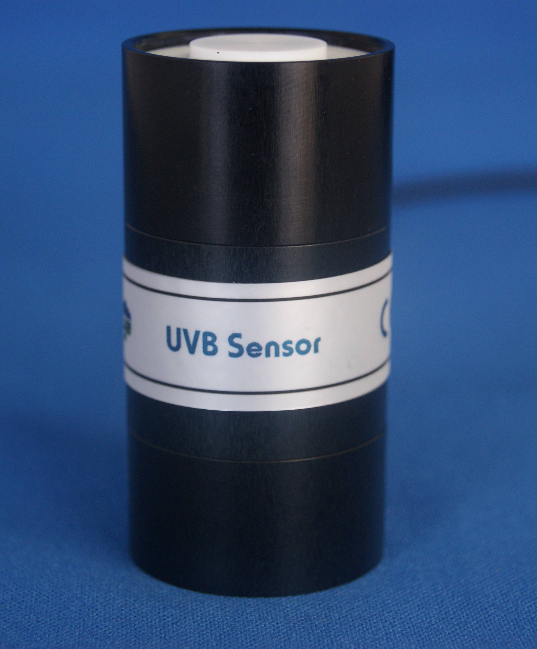{height="5cm"}
:::
### Spectral and angular (cosine) response
Radiation incident on a flat horizontal surface originating from a point
source with a defined zenith position will have an intensity value
proportional to the cosine of the zenith angle of incidence. This is
called the 'cosine law' or 'cosine-response' (see section
[9.1.2](#sec:basic:concepts:direction){reference-type="ref"
reference="sec:basic:concepts:direction"} on page ). Ideally, a
pyranometer has a directional response, which is the same as the
cosine-law. Nevertheless, directional response in a pyranometer is
influenced by the quality, dimensions and construction of the (quartz)
dome and/or Teflon diffuser. Pyranometer cosine-response is defined in
their manufacturers specification as deviation from the ideal
cosine-response using the incidence angle up to 80with respect to
1000 irradiance at normal incidence (0). Most sensors deviate
considerably from ideal cosine response at angles between 80and 90.
The erythemal response of human skin to UV radiation varies with the
individual, but for the global evaluation of UV-related health effects
to succeed, broadband measurements have to be standardized, which means
that the radiometric characteristics of all meters should be identical.
The spectral response of every meter should follow exactly the same
reference action spectrum and the angular response should not deviate
from the cosine response [@Leszczynski2002]. Hence, the spectral
response of an ideal erythemally weighted radiometer should follow the
CIE curve, and the angular response should follow the cosine function.
Unfortunately, the angular and spectral response of real erythema meters
are far from ideal; moreover, the characteristics vary from one meter
unit to another, even within the same meter type [@Leszczynski2002].
Broadband radiometers that do not follow the CIE erythemal action
spectrum as are also used. For some radiometers the spectral response
follows a bell-shaped curve centred on the UV-A or UV-B bands (see
Figure
[\[fig:UV:sensors:spectra\]](#fig:UV:sensors:spectra){reference-type="ref"
reference="fig:UV:sensors:spectra"}). Radiometers following the GEN or
other spectra commonly used as BSWFs in research with plants, are very
seldom used, and they are currently not available commercially. However,
almost any UV-B radiometer can be calibrated to measure according to
these BSWFs, but such calibrations are valid only when the calibration
light source exactly matches the spectrum of the measured light source.
::: figure*
{width="0.8\\myfigwidth"}
:::
### Calibration and intercomparison {#sec:broadband:calibration}
Each broadband instrument used to measure solar or lamp radiation should
be characterized for its spectral and angular response, and its
sensitivity to temperature (and if possible humidity). These
characteristics should be checked at regular intervals to determine
their stability. Also, correction is necessary for each instrument, as
no instrument has a spectral sensitivity identical to the erythemal
action spectrum.
To calibrate a broadband instrument for solar radiation, the basic
procedure is to simultaneously measure the spectral irradiance of the
sun with a calibrated spectroradiometer and the broadband meter under
cloudless sky conditions. The measured spectrum is weighted with the
desired spectral sensitivity[^21] of the broadband meter and integrated
over all wavelengths relevant for the broadband meter. The result is
given in the units \[detector-weighted \], relative to a defined
wavelength, usually the maximum of the erythemal action spectrum (CIE)
at 298 nm or the maximum of the spectral sensitivity of the broadband
meter. For different atmospheric conditions, such as different solar
elevation or different thickness of the ozone column, the relationship
between the detector-weighted spectral integral, measured with a
spectroradiometer, and the output of the broadband detector, after
cosine correction, should be constant within the uncertainty estimate;
if this is not the case, the mismatch indicates that the spectral
sensitivity of the broadband meter deviates from the that used to
calculate effective irradiances from the spectral irradiance data
(e.g. that defined by the CIE standard for erythema), or that the
spectroradiometric measurements were incorrectly done [@Seckmeyer2005].
When measuring the output from lamps using broadband sensors calibrated
under sunlight, large errors are incurred. In the example shown in Table
[\[tab:broadband:cal:errors\]](#tab:broadband:cal:errors){reference-type="ref"
reference="tab:broadband:cal:errors"}, we use Kipp sensors because this
manufacturer has published instrument spectral response data plotted on
a logarithmic scale. Errors of a similar magnitude should be expected
for equivalent sensors from other manufacturers. When measuring the
irradiance from lamps under a background of sunlight as in some
modulated systems, or when the spectrum changes as occurs when profiling
the radiation change with depth in water bodies, other types of
instruments like multiband sensors or spectroradiometers are preferable.
### UV radiation monitoring in growth chambers, greenhouses and phytotrons
Erythemal broadband instruments are widely used to monitor UV radiation
levels in growth chambers. Great care must be taken when using such
instruments for this purpose since plant action spectra generally
deviate from the CIE function. In addition, the reflectance of walls and
other surfaces of growth chambers may affect the readings if the cosine
response is not good. Great care is needed when artificial light sources
are used, because their spectra differ greatly from the solar spectrum
for which broadband instruments are normally calibrated. Correction
factors for the solar zenith angle and ozone dependence of the
calibration factors are based on unfiltered solar spectra, so cannot be
applied to measurements performed in such chambers, hence special
treatment of data may be necessary. In most cases if absolute readings
are needed, the broadband sensor should be calibrated against a
double-monochromator spectroradiometer, for each different light source
to be measured. Failing to do so can cause huge errors in the
measurements of doses as shown in Table
[\[tab:broadband:cal:errors\]](#tab:broadband:cal:errors){reference-type="ref"
reference="tab:broadband:cal:errors"}.
## Multi-channel filter instruments {#sec:multichannel}
Multichannel instruments are radiometers that measure a series of fixed,
usually narrow, wavelength bands of radiation. They are more rugged and
cheaper than high quality spectroradiometers and easier to deploy. Each
channel has its own detector (e.g. silicon photodiode) and filter
(e.g. interference filters). Usually there is a single diffuser acting
as common light collector for all channels. One example of a
multichannel instrument is the GUV-2511 from Biospherical Instruments
Inc (San Diego, USA) designed to measure cosine-corrected downwelling
irradiance at 305, 313, 320, 340, 380, and 395 nm, as well as PAR
(400--700 nm). When measuring daylight this allows to monitor UV
radiation in key UV wavebands for biological exposure studies. These
wavelengths also allow the extraction of cloud optical thickness and
total column ozone, two critical variables used in modelling the solar
spectrum. Multichannel sensors are mainly used for long-term monitoring
of irradiance and its geographic variation. They are also used for
ground measurements used to calibrate space-borne instruments carried by
satellites.
Recent multichannel instruments from Biospherical Instruments are
modular. They are composed of microradiometers of small size, one for
each channel, which together with input optics and filters are used to
build the multichannel instruments. Figure
[\[fig:multichannel\]](#fig:multichannel){reference-type="ref"
reference="fig:multichannel"}
::: figure*
{width="0.6\\myfigwidth"}\
{width="0.6\\myfigwidth"}
:::
The ELDONET terrestrial dosimeter consists of three broad band sensors,
measuring , and irradiance (Figure
[\[fig:ELDONET:terrestrial\]](#fig:ELDONET:terrestrial){reference-type="ref"
reference="fig:ELDONET:terrestrial"}). It uses an integrating sphere to
collect the light, which reaches the detectors after bouncing on the
sphere walls. The autonomous version includes a built-in datalogger. It
is waterproof, but it is not submersible. The underwater version is
described in section
[9.8.3](#sec:underwater:radiometers){reference-type="ref"
reference="sec:underwater:radiometers"} on page .
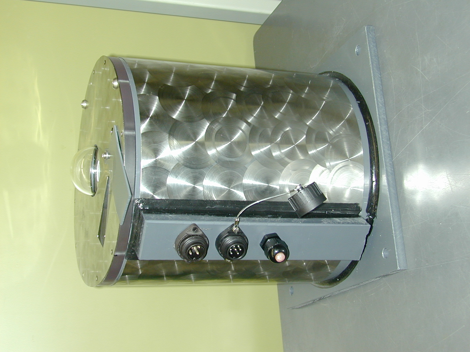
## Underwater sensors and profiling
### Measuring underwater UV radiation {#sec:underwater:measuring}
Measuring UV radiation in the aquatic environment is difficult.
Waterproof UV-measuring devices are needed or sensors protected in water
proof housings as well as a means of deploying the sensors at the
desired depth. Frequently, underwater measurements are referenced to the
(spectral) irradiance at the surface of the water body, measured
simultaneously with a matched "atmospheric" or terrestrial sensor.
As was mentioned in section [7.6](#sec:UV:aquatic){reference-type="ref"
reference="sec:UV:aquatic"} on page , measurement of the underwater UV
field presents particular complexities, mainly related to variable
attenuation occurring in different water bodies [@Kirk1994]. Depending
on the physical and chemical characteristics of the water, irradiance
may decrease much more rapidly than irradiance (this phenomenon is known
as 'spectral leakage'), resulting in a changing spectrum with depth.
Thus, underwater UV instruments are normally equipped with different
filters and photodiodes to minimize these effects and to improve the
sensitivity to particular wavelengths of interest. As discussed above in
section [9.5.4](#sec:broadband:calibration){reference-type="ref"
reference="sec:broadband:calibration"} on page , errors are introduced
if the spectrum being measured differs from that of the source used for
calibration of the broadband instrument. This implies that when using
broadband sensors underwater the errors will depend on the depth at
which the radiation is being measured. In addition, a general problem
exists for broadband sensors and spectrometers if sensors are only
calibrated in air. The same calibration function cannot be used with the
sensor in air and in water. Wavelength-dependent correction factors, so
called immersion factors, must be used to adjust the signal if sensors
are immersed in water as for example described by [@ohdet03].
Water movement and weather conditions can affect the measurements of
underwater UV radiation. For an accurate determination of UV radiation
in the field, sunny, cloudless conditions and calm waters are preferred.
The effect of waves may cause difficulties especially when measuring
near the surface. On the other hand, clouds and other atmospheric UV
absorbing phenomena can alter the conditions during the measurement of
vertical light profiles, especially when the diffuse component of the
beam is altered.
Solar zenith angle is an important factor which affects the irradiance
above the water surface, and also the reflectance of the water surface
for the wavelengths of biological relevance. In addition, the
[RAF]{acronym-label="RAF" acronym-form="singular+short"} (RAF, see also
section [\[sec:RAF\]](#sec:RAF){reference-type="ref"
reference="sec:RAF"}), can be used to estimate the effect of changes in
the ozone column on biologically effective exposure. Corrections can be
applied to measurements performed with broadband instruments, but
measurements with narrow-band multi-filter instruments and
spectroradiometers are less error prone.
If our objective is to describe the characteristics of the waters,
radiation should be measured around solar noon, when solar elevation is
maximal. However, if we are interested in describing the daily exposure
of some organism, measurements should be done preferably during most of
the day and at the depths of interest.
### Profiling {#sec:underwater:profiling}
Profiling is the measurement of irradiance or spectral irradiance as a
function of depth in a water body. Special frames are used for lowering
the instruments through the water. For light measuring instruments, the
frame or rig should not occlude the field of view of the radiation
sensors. A means of determining the depth at which the sensor is
located, and any deviation from a vertical orientation should also be
available. Suitable cabling is used to connect the underwater sensors to
onboard computers or dataloggers.
### Underwater radiometers {#sec:underwater:radiometers}
Various underwater radiometers are currently available and their
accuracy and characteristics vary considerably. The most appropriate
instrument to choose depends on the specific goals of a study. Different
types of radiometers include broadband radiometers, narrow-band
multifilter radiometers, photodiode array spectroradiometers, and
scanning spectroradiometers, including single monochromator
spectroradiometers. Comparisons of the main characteristics of different
types of instruments have been published
[@Kirk1994; @Diaz2000; @Kjeldstad2003; @Tedetti2006]. Some commonly-used
underwater instruments are described below.
The **ELDONET radiometers** (Real Time Computer, Germany) were developed
within the framework of the European light dosimeter network (Figure
[\[fig:Eldonet\]](#fig:Eldonet){reference-type="ref"
reference="fig:Eldonet"}) and have been described in detail
[@Hader1999]. The dosimeters are three-channel broadband filter devices
with an entrance optic consisting of an integrating Ulbricht sphere with
an internal BaSO$_4$ coating [@Khanh1988]. Silicon photodiodes (BPX60
for the PAR range and SFH291 for the two UV wavebands, both from
Siemens, Germany) are used in combination with custom-made filters to
select the wavelength ranges for UV-B (280--315 nm), UV-A (315--400 nm)
and PAR (400--700 nm), a custom-made interference filter for UV-B (Janos
Technology, Townshend, VT, USA), a DUG 11 band filter for UV-A (Schott &
Gen., Mainz, Germany) and a broad band filter for PAR (WBHM, Optical
Coating Laboratory, Santa Rosa, CA, USA). Eldonet performs 60
measurements each minute.
::: figure*
{width="0.6\\myfigwidth"}
:::
**Submergible multichannel radiometers** like PUV 500, PUV 2500 series
from Biospherical Instruments (San Diego, USA) are equipped with
narrow-band filter detectors in the range of UV and PAR (Figure
[\[fig:PUV\]](#fig:PUV){reference-type="ref" reference="fig:PUV"}).
These radiometers are equipped with depth and temperature sensors and
thus are well suited for accurate light profiling. The spectral
characteristics of the five filters used in the PUV 500 instrument are
as follows: 305$\pm$`<!-- -->`{=html}1 nm (band pass
7$\pm$`<!-- -->`{=html}1 nm) 320$\pm$`<!-- -->`{=html}2 nm (band pass
11$\pm$`<!-- -->`{=html}1 nm) 340$\pm$`<!-- -->`{=html}2 nm (band pass
10$\pm$`<!-- -->`{=html}1 nm) 380$\pm$`<!-- -->`{=html}2 nm (band pass
10$\pm$`<!-- -->`{=html}1 nm)
On the other hand, the PUV 2500 measures 7 (optionally 8) wavebands of
downwelling irradiance (305, 313, 320, 340, 380, 395 nm and PAR:
400--700 nm) with one upwelling radiance channel (natural fluorescence).
Each channel with 10 nm FWHHM except 305 (controlled by atmospheric
ozone cutoff). The instrument includes pressure/depth sensing (350 m
maximum) and temperature control. A 32 channel multiplexer selects
signals from 8 photodetectors, temperature, pressure and tilt/yaw
detector. The cosine collector is made of Teflon-covered quartz for use
in the water.
::: figure*
{width="0.8\\myfigwidth"}
:::
The RAMSES family of **hyperspectral radiometers** (Trios GmbH, Germany)
are miniature single monochromator spectrometers with a resolution of 2
to 3 nm per pixel and 100 or 190 usable channels in the photodiode array
(Figure [\[fig:RAMSES\]](#fig:RAMSES){reference-type="ref"
reference="fig:RAMSES"}). They can be used in air or in water. The
Ramses ACC-UV is an integrated UV hyperspectral radiometer, and the
Ramses ACC-VIS is a and visible hyperspectral radiometer, both equipped
with a cosine collector. Ramses ASC-VIS is equipped with a spherical
collector shielded so as to measure radiation from one hemisphere. To
measure scalar irradiance, two of these sensors can be deployed pointing
in opposite directions. They are calibrated for underwater and air
measurements (two different calibrations). The device has a small size,
the signal capture requires some power consumption and portable (laptop)
terminal at the surface. The detector type is a silicon photodiode array
designed to capture wavelengths between 320--950 nm for VIS models and
280--500 nm for the UV models, with an irradiance accuracy better than
6--10% depending on the spectral range.
::: figure*
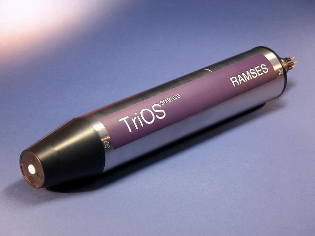
:::
Although the LI-1800UW instrument is not currently produced by LI-COR,
many foundational studies focused on UV penetration during the 1980s and
1990s were carried out using this spectroradiometer. The optics of this
scanning spectroradiometer is based on a single holographic
monochromator grating, a silicon detector and a filter wheel to improve
stray light rejection. The wavelength range is between 300 and 850 nm,
with a bandwidth of 8 nm and accuracy of $\pm$`<!-- -->`{=html}1.5 nm.
Originally optional slits of different widths were available, so these
specifications vary with the exact configuration used. The whole optical
bench and the microcomputer system is contained in the massive
waterproof housing designed for measurements to a depth close to 200 m.
Being a single monochromator instruments its accuracy is limited by
stray light when used to measure -B radiation in daylight.
::: figure*

:::
The OL 754-O-PMT Spectrometer Optics Head (Optronic Laboratories) is
based on a double monochromator for low stray light and measuring from
300 to 850 nm. Configurations with other gratings giving different
wavelength ranges are available. The system utilizes holographic
gratings with peak efficiencies at 300 nm. The instrument can be fitted
with an OL IS-470-WP Submersible Sphere Assembly (4-inch integrating
sphere) attached by means of quartz optical fibre to the non-submersible
spectroradiometer. The sphere follows a dual port design with an
entrance port and an exit port located 90$^\circ$ apart. The sphere
contains an internal baffle in front of the exit port to permit only
light reflected by internal surface of the sphere to exit the sphere and
enter the fibre.
Another approach to measuring underwater radiation is to protect a
regular sensor, as for example, those described in section
[9.5.2](#sec:broadband:instruments){reference-type="ref"
reference="sec:broadband:instruments"} on page , within a hermetic
water-proof housing (Figure
[\[fig:sensor:in:box\]](#fig:sensor:in:box){reference-type="ref"
reference="fig:sensor:in:box"}). Of course the enclosure should have an
transparent window, and the sensors must be calibrated inside the
enclosure.
## Modelling {#sec:modelling}
For locations and times not covered by measurements, alternative
approaches have to be considered for estimating the prevailing radiation
conditions. For this purpose, various methods for modelling the surface
UV radiation have been developed. These range from simple
theoretical-empirical methods for estimating the clear-sky surface
radiation to more sophisticated methods that account also for the
effects of clouds as inferred either from ground-based station data or
satellite measurements.
Table [\[tab:modelling:methods\]](#tab:modelling:methods){reference-type="ref"
reference="tab:modelling:methods"} gives a simplified view of the main
features of methods that are available for modelling the surface UV
radiation.
:::: sidewaystable*
::: center
[]{#tab:modelling:methods label="tab:modelling:methods"}
:::
[]{#methods label="methods"}
::::
Simple theoretical-empirical methods, such as those of @Bjorn1985 and
@bird1986, have been widely used thanks to their fairly simple user
interface. These methods provide spectral surface irradiances,
optionally on tilted surfaces, and account for the main parameters
affecting the surface radiation conditions under cloudless skies.
Results indicate that they predict the surface radiation with reasonable
accuracy as compared to more detailed radiative transfer calculations
and measurements [@bird1986].
Another user-friendly alternative is to use an interactive web-based
interface to radiative transfer simulations, such as the FastRT
[@engelsen2005 available at
<http://nadir.nilu.no/~olaeng/fastrt/fastrt.html>] or the QUICK TUV
(<http://cprm.acd.ucar.edu/Models/TUV/Interactive_TUV/>). Both of these
are based on rigourous radiative transfer models, which means that their
accuracy depends mainly on the choice of values for the input
parameters. Both include a selection of biological weighting functions,
and FastRT also provides the possibility to account for the effect of
clouds.
When cloud effects need to be accounted for in detail, either satellite
methods or so-called reconstruction methods should be considered. The
reconstruction methods usually rely on ground-based measurements of some
kind for accounting for the effect of clouds on radiation. Although the
methods vary in their exact approach, the idea of all of them is to
utilize available observations to account for the parameters that affect
the amount of UV radiation reaching the surface. These parameters are,
most importantly, clouds, total ozone column, surface albedo,
atmospheric aerosols, and altitude or pressure. In addition, the solar
zenith angle determines the path length of the
[direct:rad]{acronym-label="direct:rad" acronym-form="singular+short"}
through the atmosphere and is therefore the single most important factor
for the surface UV radiation. The Earth-Sun distance, which varies over
the course of the year, also needs to be accounted for.
Many station-based methods for reconstructing the surface radiation were
included in recent European efforts to gain a better understanding of
past radiation and its climatological behaviour
[@kopke2006; @denouter2010]. Similar methods have been proposed and
applied in other parts of the world as well
[@fioletov2001; @fioletov2004]. Compared to satellite methods, the
advantage of the station-based methods is that they tend to give more
accurate estimates of the surface UV radiation. In particular, methods
using (300--3000 nm), measured by pyranometers at numerous stations
worldwide, as input for determining the cloud effect typically show
small bias and fairly small scatter when compared to measurements
[@kopke2006]. To mention one example, @lindfors2007 estimated daily
erythemal UV doses at four Nordic stations, and found a systematic
difference of between 0 and 4%, depending on the station, and a
root-mean-square error of 5--9% as compared to measurements for the
summer period.
Satellite methods are based on radiative transfer simulations combined
with information on, for example, clouds and total ozone column
retrieved from the satellite observations. Satellite retrieved UV
irradiances typically show an overestimation of 10% or more, and a large
scatter, when compared to surface measurements: the root-mean-square
errors for daily erythemal UV doses tends to be of the order of 30--40%
[@kujanpaa2010; @tanskanen2007; @lindfors2009b]. The main part of the
overestimation is usually attributed to aerosol absorption, which is not
accounted for properly in current satellite UV algorithms. The advantage
of satellite methods, on the other hand, is their large geographical
coverage, often global, and easy access to data that they provide.
Most methods, both station-based UV reconstruction methods and satellite
methods, only provide UV data corresponding to a selection of weighting
functions (e.g., erythemally weighted ), and, in addition, sometimes
irradiances for selected wavelengths. Furthermore, the methods typically
include only irradiances for a horizontal surface. This may become an
obstacle for biological applications where, for example, a specific
weighting function or spectral information would be preferred. In
principle, however, many of the methods could be extended to produce
spectral irradiances and fluence rates. On the other hand, fluence rates
can also be estimated based on the horizontal irradiance [e.g.,
@kylling2003].
Recently, @lindfors2009 presented a method for modelling spectral
surface irradiances. The method relies on radiative transfer
simulations, and takes as input (1) the effective cloud optical depth as
inferred from pyranometer measurements of
[global:rad]{acronym-label="global:rad" acronym-form="singular+short"};
(2) the total ozone column; (3) the surface albedo as estimated from
measurements of snow depth; (4) the total water vapour column; and (5)
the altitude of the location.
Figure [\[fig:jok2001\]](#fig:jok2001){reference-type="ref"
reference="fig:jok2001"} shows a comparison between the daily
accumulated irradiances at 300 and 320 nm from this method and
measurements with a Brewer spectroradiometer at Jokioinen, southern
Finland. At both wavelengths, the reconstructed irradiances closely
follow the measured ones.
::: figure*

:::
A variety of methods for modelling the surface UV radiation are
available. Which method is the best, or the most appropraite, depends on
the specific question that is to be answered. In general, the complexity
of the method tends to grow with increasing accuracy, and the
pyranometer-based UV reconstruction methods, that are considered to
provide highest accuracy, typically require an expert user. The use of
such a method will, however, increase cross-disciplinary collaboration
and may therefore be worthwhile.
::: example*
[]{#ex:effective:irradiance label="ex:effective:irradiance"} By
'biologically effective irradiance' we mean the irradiance weighted
according to the effectiveness of different wavelengths in eliciting a
photobiological response. The most frequently used biologically
effective irradiance quantities are photometric quantities such as those
described in Box
[\[box:photometric:quantities\]](#box:photometric:quantities){reference-type="ref"
reference="box:photometric:quantities"} on page . In the case of
photometric quantities the (energy) irradiance is weighted according to
the response of the human eye.
When studying the effects of radiation on plants we use as
[BSWFs]{acronym-label="BSWF" acronym-form="plural+short"} (BSWFs)
spectra describing the response of some plant function. For example an
action spectrum for accumulation of flavonoids, or an action spectrum
for growth inhibition. To be able to calculate biologically effective
irradiances using any BSWF, we need to measure the spectral irradiance
of the light source.
If we integrate the effective irradiance for the duration of an
experiment then we obtain a biologically effective exposure (usually
called 'biologically effective dose' by biologists). If we do the time
integration for one day we obtain a biologically effective daily
exposure.
These weighted irradiances are usually expressed using units
corresponding to the underlying energy irradiances, independently of the
BSWF used. Quantities calculated using different BSWFs are expressed in
the same units, but the values cannot be compared because in reality
they are measured on different scales.
:::
## BSWFs and effective UV doses {#sec:BSWFs:UVeff}
The emission spectrum of UV-B lamps, even filtered with acetate, is
different to that of the effect of ozone depletion. The spectrum of the
effect of ozone depletion not only changes with ozone column thickness,
but also with solar elevation. In other words, it changes through a day
and with seasons (Figure
[\[fig:lamp:solar:spectra\]](#fig:lamp:solar:spectra){reference-type="ref"
reference="fig:lamp:solar:spectra"}). Because of this, it is almost
impossible to exactly simulate the effect of ozone depletion in field
experiments. The best we can do is to calculate effective doses.
::: figure*

:::
Biologically effective exposures (see Box
[\[ex:effective:irradiance\]](#ex:effective:irradiance){reference-type="ref"
reference="ex:effective:irradiance"}) are a way of measuring radiation
differing in spectral composition with the same 'measuring stick'. This
'measuring stick' is a biological response. Behind each measurement we
need to assume the involvement of a biological response. If we know the
action spectrum for the biological response, we can use it as a BSWF: We
multiply, wavelength by wavelength the spectral irradiance of the light
source by the BSWF obtaining a weighted spectrum, giving a
biologically-effective *spectral* irradiance (Figure
[\[fig:eff:spectral:irrad\]](#fig:eff:spectral:irrad){reference-type="ref"
reference="fig:eff:spectral:irrad"}). We then integrate the result over
wavelengths, to obtain a single number, the biologically effective UV
irradiance[^26]. In Figure
[\[fig:eff:spectral:irrad\]](#fig:eff:spectral:irrad){reference-type="ref"
reference="fig:eff:spectral:irrad"} it also possible to appreciate the
difference in relative change of this effective irradiance, for a given
level of ozone depletion, depending on the BSWF used.
It is important to make sure that both the irradiance and the
effectiveness are measured using compatible units. It is common to
express action spectra as spectral *quantum* effectiveness and to
measure light sources as spectral (*energy*) irradiance. In research,
biologically effective doses are most frequently expressed in weighted
energy units and to be able to calculate these doses from spectral
(energy) irradiance measurements for a light source (sunlight or lamps)
one needs to use an action spectrum expressed in energy effectiveness.
Most common formulations of action spectra need to be transformed from
quantum effectiveness to energy effectiveness (one important exception
is the CIE erythemal spectrum formulation). This is something that is
often neglected, and is a source of difficulties when comparing doses
between different publications.
Another possibility for measuring effective doses is to have a broadband
sensor with a spectral response resembling the action spectrum of
interest. In practice the spectral response of such sensors is only an
approximation to the desired and consequently need to be calibrated
under the light source to be measured, usually by comparison to a double
monochromator scanning spectroradiometer (see section
[9.7](#sec:spectroradiometers){reference-type="ref"
reference="sec:spectroradiometers"} on page ). Most such sensors are
calibrated for sunlight, and consequently give biased readings when used
for measuring radiation from most lamps.
::: figure*

:::
[]{#sec:RAF label="sec:RAF"}The [RAF]{acronym-label="RAF"
acronym-form="singular+short"} () gives the percent change in effective
dose () or, strictly speaking, effective exposure () for each percent
change in ozone column thickness. It should be calculated using
logarithms. $$\mathrm{RAF} = \frac{\ln \dose[d] - \ln \dose[n]}%
{\ln [\Chem{O_3}]^\mathrm{n} - \ln [\Chem{O_3}]^\mathrm{d}}$$
where is dose and $[\Chem{O_3}]$ ozone concentration, and superscript
$\mathrm{d}$ indicates ozone depleted condition, and superscript
$\mathrm{n}$ indicates normal, or reference, ozone depth condition. The
value of depends strongly on the action spectrum used to calculate the
effective dose. Looking at
fig. [\[fig:eff:spectral:irrad\]](#fig:eff:spectral:irrad){reference-type="ref"
reference="fig:eff:spectral:irrad"}, it can be understood why is much
larger for GEN than for PG.
### Weighting scales
Ultraviolet action spectra are usually normalized to quantum
effectiveness = 1 at 300 nm. This is arbitrary, and especially in the
older literature, you will find action spectra normalized at other
wavelengths. In the Materials and Methods section always report the
normalization used, in addition to the action spectrum used as a BSWF.
Remember that as the wavelength used for normalization is arbitrary,
values of effective UV doses calculated using the same BSWF but
normalized at different wavelengths cannot be directly compared because
they are expressed on different scales. Of course biologically effective
irradiances based on different BSWFs cannot be compared to each other
either.
Using the correct BSWF is very important, as using the wrong BSWF has
usually serious implications on the interpretation of experimental
results [@Caldwell2006; @Kotilainen2011].
### Comparing lamps and solar radiation
Frequently we want to compare UV doses in growth chambers to doses
outdoors. Unless we have a solar simulator the spectra will differ
significantly. It is especially important to keep the ratio similar to
that in solar radiation. Table
[\[tab:UVeff\]](#tab:UVeff){reference-type="ref" reference="tab:UVeff"}
gives an example comparing a frame with two acetate-filtered Q-Panel
UVB-313 lamps to sunlight with normal and 20% depleted ozone at
Jokioinen for 21 May at 11:30.
### Effective doses, enhancement errors and UV-B supplementation {#sec:enhancement:errors}
Ultraviolet-radiation supplementation can be modulated so as to follow
natural variation in solar UV or just follow a daily square wave pattern
(see section [8.2.6](#sec:modulated){reference-type="ref"
reference="sec:modulated"} on page ). It is important that lamps are
filtered with cellulose di-acetate film (to remove UV-C radiation
emitted by UV-B lamps, which is absent in natural sunlight) and that
these filters are replaced regularly, specially in the case of square
wave systems, as modulated systems with feedback compensate for the
reduced dose automatically (although not for the change in spectrum)
[@Newsham1996a]. Even when adequately filtered the emission spectrum of
UV-B lamps does not match the effect of depletion (Figure
[\[fig:weighted:lamp:depl:GPAS:PG\]](#fig:weighted:lamp:depl:GPAS:PG){reference-type="ref"
reference="fig:weighted:lamp:depl:GPAS:PG"}. We need to calculate
effective doses using BSWFs.
::: figure*

:::
Errors caused by the mismatch between the doses aimed at and those
achieved when simulating the effect of ozone depletion with UV-B
enhancement with lamps are called enhancement errors. The main source of
these errors is the mismatch between the assumed spectral response and
the real spectral response. This is so because the adjustment of the
burning time (or power) of the UV-B lamps used for enhancement needs to
be based on biologically effective doses. However, depending on the
different BSWFs used, the needed lamp burning time may be long or short
(Figure
[\[fig:lamp:burning:times\]](#fig:lamp:burning:times){reference-type="ref"
reference="fig:lamp:burning:times"}). Another way of looking at this
problem is to compare the deviation of the achieved when using a
'wrong'[^27] BSWF compared to the target one---e.g. corresponding to a
certain magnitude of ozone depletion. Figure
[\[fig:achieved:CIE\]](#fig:achieved:CIE){reference-type="ref"
reference="fig:achieved:CIE"} shows this comparison for the frequent
case of use of a CIE-weighted broadband sensor to control the lamps used
in experiments with plants. The errors are surprisingly small for GEN
and PG.
::: figure*

:::
::: figure*

:::
An additional source of errors is shading by the lamp frames. If we do
not attempt to compensate for the shade with UV-B from the lamps the
error between PG and GEN is small [@Kotilainen2011]. How much the
effective UV dose decreases with shading does not depend on the BSWF
used as long as the shade is 'gray' (equally affects all relevant
wavelengths). However, how much UV from the lamps will be needed to
compensate for this will depend on the BSWF used (Table
[\[tab:shading:errors\]](#tab:shading:errors){reference-type="ref"
reference="tab:shading:errors"}). With some BSWFs the lamp power or
burning time needed to compensate for shading is much more than that
needed to simulate ozone depletion, because with spectra like PG, we
need to replace shaded UV-A with UV-B from lamps. See section
[\[sec:RAF\]](#sec:RAF){reference-type="ref" reference="sec:RAF"} on
page for a discussion of the relationship between changes in ozone
column and changes in effective UV radiation.
To minimize shading errors we must build lamp frames that produce little
shade. Probably $<\!5$% shading is achievable. We should not attempt to
compensate for shading by the frames with UV from lamps. Shifting the
whole experiment's UV baseline dose by a small percentage but keeping
the size of enhancement at the target level is probably the best
approach available.
## Effective UV doses outdoors: seasonal and latitudinal variation
The state of the atmosphere (in terms of ozone column thickness,
cloudiness and aerosol content) together with day-length and daily
course of the solar zenith angle () are the main factors determining the
climatology of (and its components, and ) at ground level. For clear sky
conditions the average spatial and temporal distribution of UV
irradiance can be computed by means of a radiative transfer model fed
with proper and aerosol data [@Grifoni2008; @Grifoni2009]. In these
conditions the latitudinal and temporal distribution of irradiance are
driven mainly by two factors: day-length and through the day. See
section [9.9](#sec:modelling){reference-type="ref"
reference="sec:modelling"} on page for a discussion of different
approaches to modelling.
To go from the climatology of spectral irradiance to that of the
biologically effective () exposures (or doses), spectral irradiance has
to be weighted to account for the different efficiency of each
wavelength in producing biological effects; this is done applying a
BSWF---based on the action spectrum of the biological process
considered. Plant action spectra differ in the weight given to and
radiation, as it has been illustrated in section
[7.8](#sec:action:spectra){reference-type="ref"
reference="sec:action:spectra"} on page . In this analysis @Grifoni2009
considered two action spectra related to plant response: the so-called
Generalized Plant Action spectrum [GEN, proposed by @Caldwell1971] and
the more recent Plant Growth spectrum [PG, @Flint2003a]. The erythemal
action spectrum [CIE, @McKinlay1987] was also included since instruments
with a spectral sensibility quite close to it have been used in several
field experiments. The analysis presented in this section was based on
spectral global irradiance for cloud-free conditions on horizontal
surfaces simulated by means of the STAR model
[@Ruggaber1994; @Schwander2000] for Rome, Italy (lat. 41.88 N,
long. 12.47 E), Potsdam, Germany (lat. 52.40 N, long. 13.03 E) and
Trondheim, Norway (lat. 63.42 N, long. 10.42 E) on the first day of each
month of the year from 1:00 to 23:00 (UTC time) with a 30 min time step.
Daily doses () were calculated for all these 12 days.
After convoluting the spectral energy irradiances at ground level for
the three locations and seasons with the three BSWFs, a picture of the
seasonal of radiation was obtained, which was different depending on
latitude. The pattern of seasonal and latitudinal variation of the daily
doses is shown to depend strongly on the BSWF, and day of the year
(Table [\[tab:doses:seasons\]](#tab:doses:seasons){reference-type="ref"
reference="tab:doses:seasons"}).
The changes in daily doses occurring through the year relative to the
yearly average, for the three locations across Europe illustrate the
effect of action spectra used as BSWFs (Figure
[\[fig:doses:seasonal\]](#fig:doses:seasonal){reference-type="ref"
reference="fig:doses:seasonal"}).
::: figure*

:::
The largest seasonal variation occurs when the daily doses are computed
on the basis of action spectra completely or partially excluding the
contribution of the component, as in the case of GEN and CIE
respectively. Figure
[\[fig:doses:seasonal\]](#fig:doses:seasonal){reference-type="ref"
reference="fig:doses:seasonal"} shows the extent to which latitude
affects these seasonal changes, which have a larger amplitude as the
latitude increases. In other words, the climatology of appears to be
strongly dependent on the action spectrum used, and, as different plant
responses follow different action spectra, the effective climatology
will depend on the plant response under study.
These differences in climatology are ecologically relevant, for instance
for perennial species that may experience different seasonal change in
the irradiance they are exposed to, depending on the latitude at which
they are growing and on the biological process/action spectrum studied.
## Effective UV doses in controlled environments
If the light spectrum in a controlled environment differs greatly from
that under natural conditions, the relative biologically effective
irradiances will differ greatly depending on the action spectrum used as
. For example, if irradiance is much lower in daylight than in the
controlled environment, but irradiance similar to that in daylight, the
dose calculated using GEN(G) as a BSWF will differ little between the
controlled environment and daylight, but the dose based on PG will be
much lower in the controlled environment than in daylight. This example
shows why we need to use a realistic light spectrum in controlled
environments when we want to extrapolate the results from such
experiments to natural conditions. Furthermore, an increased ratio
between and radiation, and/or radiation and artificially enhances the
responses of plants to radiation.
## An accuracy ranking of quantification methods
Table
[\[tab:methods:accuracy\]](#tab:methods:accuracy){reference-type="ref"
reference="tab:methods:accuracy"} shows a preliminary comparison of
different methods available for quantifying solar UV radiation and
estimating biologically effective doses. Bias is the systematic
directional deviation from the true value, for example overestimation of
irradiance or doses. Uncertainty is a random deviation that prevents us
from knowing the true value, but deviations are not systematic
---measurements from different instruments or the same instruments after
different recalibrations will deviate by different amounts and in
different directions from the true value.
A detailed comparison is difficult with the information currently
available, consequently some gaps remain in the table. However, some
general recommendations are possible. For outdoors experiments with
manipulation of solar , the best option is most probably a combination
of (a) hourly simulation of UV spectral irradiance with a model using
ground station data as input, plus (b) spot measurements, for example
under different filters with a spectroradiometer under clear sky
conditions. It is best to replace modelling (a) with actual continuous
measurements with a well calibrated double monochromator
spectroradiometer. However, this is rarely possible in practice, as
there are few ground stations producing validated spectral data.
For experiments using lamps, the best option from the point of view of
accuracy is the use of a double monochromator spectroradiometer. From a
practical viewpoint, using a broadband instrument calibrated against a
double monochromator spectroradiometer, may be easier. When measuring
mixed daylight and lamp radiation, or mixed radiation from diverse
lamps, or when there is degradation of filters, broadband instruments
are totally unsuitable.
Single monochromator spectroradiometers should be avoided for
measurements of radiation when there is a background of or visible
radiation, unless very special handling of stray light is done by a
combination of special measuring protocols and data processing.
::: table*
:::
## Sanity checks for data and calculations {#sec:sanity:quantifying}
When quantifying radiation, or in fact when doing any measurement, one
should compare the values (e.g. irradiances or daily doses) against what
has earlier been reported in the literature for a similar light source.
In this way many errors can be detected. To help in this process we
present in Table
[\[tab:typical:irrad:values\]](#tab:typical:irrad:values){reference-type="ref"
reference="tab:typical:irrad:values"} typical values for both unweighted
and (energy) irradiance, photon irradiance, and biologically effective
irradiances with the most frequently used BSWFs and wavelength
normalisations. For radiation outdoors one can use a model (e.g. TUV
quick simulator) to estimate spectral irradiance values and from them
calculate effective doses or exposure. We have done these calculations
for some sites, and present them in Table
[\[tab:typical:irrad:values\]](#tab:typical:irrad:values){reference-type="ref"
reference="tab:typical:irrad:values"}. We have also included data for
some lamps.
## {#sec:recommend:quantifying}
In this section we list recommendations related to the quantification of
radiation in experiments. See sections
[8.6.1](#sec:recommend:outdoor:manip){reference-type="ref"
reference="sec:recommend:outdoor:manip"} and
[8.6.2](#sec:recommend:indoor:manip){reference-type="ref"
reference="sec:recommend:indoor:manip"} for recommendations on
manipulation of radiation, section
[10.9](#sec:recommend:grow){reference-type="ref"
reference="sec:recommend:grow"} for recommendations about plant growing
conditions, and section
[11.12](#sec:recommend:stat){reference-type="ref"
reference="sec:recommend:stat"} for recommendations about statistical
design of experiments.
1. Always report in your publications the radiation effective exposure
(frequently called effective doses in the biological literature),
depending on the type of experiment, as daily integrated values or
effective irradiances plus daily exposure time. Calculate effective
doses using relevant action spectra and if possible report doses
using all the most commonly used ones: CIE, GEN(G), and PG.
2. Always indicate the name of the quantity measured, the type of
sensor and its position during measurement, location of sensor with
reference to plants, and unit of measurement. In the case of
effective doses, indicate how they were calculated, in particular,
cite the bibliographic source for the action spectrum and
formulation used, and at which wavelength the spectrum was
normalized to effectiveness equal to unity.
3. Whenever possible include in your publications the emission spectrum
of the light source and/or transmittance spectrum of the filters
used, or cite an earlier paper where the spectra have already been
published.
4. Use only instruments with recent and valid calibration data for the
measurements at hand.
5. Make sure, in the case of broadband sensors, that the calibration is
valid for the light source being measured. For example, broadband
sensors calibrated for sunlight should **not** be used for measuring
irradiance under lamps.
6. If high precision is required in the measurements, apply all the
necessary corrections. This is important both for broadband and
spectral measurements.
7. Be aware of temperature effects on the functioning of the meter and
sensor used and apply the required corrections or use temperature
stabilized instruments.
8. Single monochromator array or scanning spectrometers can be used for
measuring effective exposures in sunlight only with very serious
limitations and only if complicated corrections are applied to the
raw data to take into account stray light and the properties of the
slit function. These corrections are not possible with the software
provided by the makers of the instruments. Uncorrected measurements
from this type of instruments are subject to huge uncertainties and,
what is worse, bias. Use double monochromator spectroradiometers
instead.
9. When using spectrometers configured with SMA connectors for optical
fibres, do not detach the fibre at the spectrometer end[^28][^29].
Doing so invalidates the calibration because the alignment of the
fibre with respect to the entrance slit may be different after the
fibre is reattached.
10. When measuring, take into account the field of view of the entrance
optics of your instrument (e.g. one hemisphere for a cosine
corrected irradiance sensor) and make sure that yourself and any
other nearby objects do not disturb the radiation 'seen' by the
instrument.
11. Take into account that spot measurements of in sunlight under
different filters describe only one point in time. Continuous
measurements or modelling based on continuous ground-based
measurements are needed to fully describe the treatments applied.
12. Outdoor irradiance is affected by cloudiness, so measurements where
a single instrument is moved to take sequential measurements under
the different treatments should be avoided unless the sky is
perfectly clear. In addition, parallel measurement of PAR or global
radiation in the open is recommended so as to be able to detect any
variation due to clouds.
13. exposure values (also called doses) derived from satellite-based
measurements are subject to relatively large errors and bias, so it
is better to avoid their use, specially when daily or weekly values
are needed. Much of the uncertainty derives from the sparse nature
of the satellite data (e.g. one or fewer fly overs per day).
14. Routinely check your instruments. Frequently check that the readings
are very close to zero when the sensor is in darkness. Do sanity
checks on your data against values expected (e.g. using models or
published data). For example if when measuring a sunlight spectrum
you get spectral irradiance values different from zero[^30] at
wavelengths shorter than 290 nm you can be sure that there is a
problem. There may be too much stray light, or a bad correction for
the dark signal, or simply the spectrometer is not good enough for
the job.
15. When measuring sunlight or lamp spectra for calculating effective
doses you need a spectroradiometer with a spectral resolution of at
least 1 nm. Furthermore to reduce noise use only averaging of
repeated scans rather than 'Boxcar smoothing'. Boxcar smoothing
reduces the spectral resolution by doing a moving average across
wavelengths.
## Further reading {#further-reading-1}
### UV climatology and modelling
<http://cprm.acd.ucar.edu/Models/TUV/Interactive_TUV/>\
<http://zardoz.nilu.no/~olaeng/fastrt/>\
<http://jwocky.gsfc.nasa.gov/teacher/ozone_overhead.html>
### Instrumentation and UV measurement validation
The report [@Bentham1997] describes scanning spectroradiometers. It is
available at <http://www.bentham.co.uk/pdf/UVGuide.pdf>. The report
[@Seckmeyer2010] gives guidelines for the use of array spectrometers for
measuring radiation. This report is available at
<http://www.wmo.int/pages/prog/arep/gaw/documents/GAW191_TD_No_1538_web.pdf>.
The report [@Seckmeyer2010a] is available at
<http://www.wmo.int/pages/prog/arep/gaw/documents/GAW190_TD_No_1537_web.pdf>.
The report [@Seckmeyer2005] is available at
<ftp://ftp.wmo.int/Documents/PublicWeb/arep/gaw/final_gaw164_bookmarks_17jul.pdf>,
while the first report of the series, titled [@Seckmeyer2001] is only
available in printed form.
### Books
The book edited by @Diffey1989 includes information on detectors and
methods not described in this handbook, or that are described here in
less detail.
## Appendix: Formulations for action spectra used as BSWFs {#app:formulations}
The calculation of biologically effective UV doses requires weighting
the spectral energy irradiance () or spectral photon irradiance () at
each wavelength with a weighting value that is typically generated from
a mathematical formulation fitted to describe the weighting function or
action spectrum of the biological process---i.e. a
[BSWF]{acronym-label="BSWF" acronym-form="singular+short"} (BSWF). Data
obtained from a spectroradiometer are usually provided as spectral
energy irradiance (units: ) and care should be taken to use the
appropriate formulation that uses either energy effectiveness () or
quantum effectiveness () values as appropriate.
The usual approach is to base effective UV doses on energy irradiance
data, using BSWFs that provide values for relative energy effectiveness
at each wavelength. However, BSWFs are often defined using quantum
effectiveness for application to photon irradiance values. Consequently,
conversion of energy irradiance values measured during experiments to
photon irradiance is necessary before applying weighting functions
originally formulated using quantum effectiveness. Conversion of energy
irradiance values to photon irradiance can be achieved using equation
[\[eq:photon\]](#eq:photon){reference-type="ref" reference="eq:photon"}
on page . After conversion, the calculated effective doses will be on a
different scale than if they are calculated based on energy irradiance
values. Note that you may find examples in the literature where
formulations based on quantum effectiveness () have been inappropriately
applied to spectral energy exposure (unit: ) or spectral energy
irradiance (unit: ).
The general plant action spectrum of Caldwell (Code GEN in Table
[\[tab:action:spectra\]](#tab:action:spectra){reference-type="ref"
reference="tab:action:spectra"} on page ) was originally published
simply as a graphical figure of quantum effectiveness against wavelength
[@Caldwell1971] and subsequently two publications have fitted different
mathematical formulations to describe its use as a weighting function.
@Green1974 fitted a function that decreases to zero at 313 nm whereas an
alternative mathematical fit provided by @Thimijan1978 continues to
weight irradiance values up to 345 nm in the region. Both of these
functions are shown on Figure
[\[fig:action:spectra\]](#fig:action:spectra){reference-type="ref"
reference="fig:action:spectra"} on page as GEN(G) and GEN(T)
respectively. It is important to specify which mathematical function has
been used when describing the calculation of effective UV doses in
experimental methods.
The general plant action spectrum of Caldwell fitted with the
mathematical function of @Green1974 is given by [Source: @Bjorn1993a]:
$$\qeff[GEN(G)](\lambda) = \begin{cases}
2.618 \cdot \left[ 1-\left(\frac{\lambda}{313.3}\right)^2 \right] \cdot %\cr
\mathrm{e}^{-\frac{\lambda-300}{31.08}} & \text{if $\lambda\le313.3$ nm}\\
0 & \text{if $\lambda>313.3$ nm}
\end{cases} \label{eq:GEN.G}$$
and when fitted with the mathematical function of @Thimijan1978 is given
by [Source: @Bjorn1993a]:
$$\qeff[GEN(T)](\lambda) = \begin{cases}
\mathrm{e}^{-\left(\frac{265-\lambda}{21}\right)^2} & \text{if $\lambda\le345$ nm}\\
0 & \text{if $\lambda>345$ nm}
\end{cases} \label{eq:GEN.T}$$
The DNA damage formulation of @Green1975 is given by:
$$%\qeff[DNA(GM)](\lambda) & = & \exp\left\{ 13.82 \cdot \left[ \left( 1+\exp\left( \frac{\lambda-310}{9} \right)\right)^{-1} -1 \right] \right\} \label{eq:DNA.GM}
\qeff[DNA(GM)](\lambda) = \mathrm{e}^{ 13.82 \cdot \left[ \left( 1+\mathrm{e}^{ \frac{\lambda-310}{9}} \right)^{-1} -1 \right] } \label{eq:DNA.GM}$$
The doses calculated with this formulation differ significantly from
doses calculated using tabulated values derived from the figure in
@Setlow1974. For example the model TUV and the data from the NSF
monitoring network use the tabulated values rather than the formulation
by @Green1975.
However, most BSWFs are conventionally used with a value of one at 300
nm. This may be achieved by simple calculation adjustments within a
spreadsheet (by dividing each wavelength effectiveness by the
effectiveness value at 300 nm) or by altering the mathematical formula
directly. Thus, the mathematical formulation of @Green1974 for GEN(G)
requires equation [\[eq:GEN.G\]](#eq:GEN.G){reference-type="ref"
reference="eq:GEN.G"} to be multiplied by 4.596 to normalize it to a
value of 1 at 300nm and similarly GEN(T) requires equation
[\[eq:GEN.T\]](#eq:GEN.T){reference-type="ref" reference="eq:GEN.T"} to
be multiplied by 16.083 and DNA(GM) requires equation
[\[eq:DNA.GM\]](#eq:DNA.GM){reference-type="ref" reference="eq:DNA.GM"}
to be multiplied by 30.675.
The formulation of the weighting function published by @Flint2003a for
plant growth, shown as PG in Figure
[\[fig:action:spectra\]](#fig:action:spectra){reference-type="ref"
reference="fig:action:spectra"} on page , was for quantum effectiveness
and already provides normalization to 1 at 300 nm and is given by:
$$%\qeff[PG](\lambda) & = & \cases{\mathrm{e}^{4.688272\ \cdot
% \mathrm{e}^{-\mathrm{e}^{0.1703411 \cdot \frac{\lambda-307.867}{1.15} +
%\left(\frac{390-\lambda}{121.7557}-4.183832\right)}}} & if $\lambda\le390$ nm\cr
%0 & if $\lambda>390$ nm\cr} \label{eq:PG}
\qeff[PG](\lambda) = \begin{cases}\exp\left(4.688272\ \cdot \right. \cr
\left.
\ \ \ \exp\left(-\exp\left(0.1703411 \cdot \frac{\lambda-307.867}{1.15}\right)\right) + \right. %\cr
\left.
\left(\frac{390-\lambda}{121.7557}-4.183832\right)\right) & \text{if $\lambda\le390$ nm}\\
0 & \text{if $\lambda>390$ nm}
\end{cases}
\label{eq:PG}$$
Some weighting functions are already defined using energy effectiveness
values for use with energy irradiance data, one example being the CIE
erythemal action spectrum [@McKinlay1987; @Webb2011]. The standard was
revised in 1998 and the updated version should be used instead of the
original one from 1987 [@Webb2011]. It is important to check that
published mathematical formulae have been appropriately normalized to
one at 300 nm. However, whereas most BSWFs are conventionally set to one
at 300 nm, the CIE98 erythemal weighting function has defined values at
specific wavelengths [@Webb2011] and is given by:
$$\eeff[CIE](\lambda) = \begin{cases}
1 & \text{if $250\le\lambda\le298$ nm}\\
10^{0.094(298-\lambda)} & \text{if $298\le\lambda\le328$ nm}\\
10^{0.015(140-\lambda)} & \text{if $328\le\lambda\le400$ nm}\\
0 & \text{if $\lambda > 400$}
\end{cases} \label{eq:CIE}$$
Weighting functions defined using quantum effectiveness (), and
normalized to one at 300 nm, can be converted to relative energy
effectiveness () simply by multiplication, wavelength by wavelength, of
the quantum effectiveness by by the respective wavelength in nm and
dividing by 300 (the chosen normalization wavelength in nm). The value
300 should be changed when using other wavelengths for normalization.
This is based on equation
[\[eq:photon\]](#eq:photon){reference-type="ref" reference="eq:photon"}
giving the energy in one photon, but as Planck's constant ($h$) and the
speed of light in vacuum ($c$) are constant divisors, and we are
expressing the effectiveness in relative units, they can be left out of
the calculation.
It is always essential to specify clearly the normalization wavelength,
the mathematical formulation and the BSWF used when describing the
calculation of effective UV doses.
:::::::: multicols
2
## Appendix: Calculation of effective doses with Excel {#app:Excel}
Let us start with a text file generated by a spectroradiometer and its
connected computer. With the instruments that I have used this text file
consists of one column, containing either spectral (energy) irradiance
or spectral photon irradiance (some instruments, especially for
underwater use, may have fluence rate instead of irradiance). At the
start, above the columns, is a heading containing supplementary
information. Other instruments may have two columns, the first one
containing wavelength values, the other one spectral irradiance values.
For the Optronics instruments that I have used, the start of a data file
looks like the listing in Figure
[\[fig:list:Optronics\]](#fig:list:Optronics){reference-type="ref"
reference="fig:list:Optronics"}. The heading here contains "a", which in
this case is the name of the file, the kind of data that is recorded
(including the unit), the date, the starting wavelength in nm, the end
wavelength (not shown here) in nm, and the step interval in nm. This
file can be loaded into an Excel file going to
`Data`$>$`Get external data`$>$`Load text file`. When you have done
this, insert a new column to the left of the one containing the measured
data. In this new column you should fill in the wavelength values, which
can be done in the following way without typing every value:
:::: figure*
::: footnotesize
"a","Irradiance [W/(cm^2 nm)]",971217,250.00,400.00,1.00
1.439562E-010
1.797497E-010
6.126532E-010
4.516362E-009
8.027722E-009
1.081851E-009
2.862175E-010
1.728253E-010
1.790998E-010
1.953554E-010
2.570309E-010
...
:::
::::
Type the first two values, i.e. in this case first "250" in the cell
left of the one containing the first radiation value 1.439562E-010.
Since the step interval is 1.00 nm, the next value is 251. Type this in
the cell to the left of the value 1.797497E-010. Select the two cells
that you have just filled in. Put the cursor at the lower left corner of
the cell containing "251" and see it change appearance, push the (left)
mouse button and drag down to the cell left of the last radiation value.
The column will then fill up with the appropriate wavelength values.
You have now filled columns A and B with the appropriate values. Next
you should generate a column with values of the weighting function.
Suppose you wish to use the weighting function of @Flint2003a. The
formula given for this in the publication is Biologically effective UV=
$\exp[4.688272*\exp(- \exp(0.1703411*(x-307.867)/1.15))+((390-x)/121.7557-4.183832)]$
in which $x$ stands for wavelength in nm.
Select cells in column C over the rows corresponding to values in
columns A and B. Go to "Tools" on top of the file, push the mouse button
and go down and select "Calculator". Type the formula above, with the
exceptions that you use ordinary parentheses instead of square brackets,
"A:A" instead of "x" (do not type the quotation marks), and comma
instead of dot if you use the comma system. When this is done, press OK
and save the result.
You now have the values of the weighting function in column C. If you
double-click on the first value in column C you should get the equation
entered. The top of your file should then look like Figure
[\[fig:Excel:sheet\]](#fig:Excel:sheet){reference-type="ref"
reference="fig:Excel:sheet"}. If you insert a new column C to the left
of your old column C and copy the wavelength values into it you can plot
your weighting function as a check. If you plot it on a logarithmic
abscissa, it should look something like Figure
[\[fig:Excel:PG\]](#fig:Excel:PG){reference-type="ref"
reference="fig:Excel:PG"}. This can be compared to the plot in the
original publication by @Flint2003a. Once you have generated a weighting
function that you wish to use several times, you need of course not
calculate it like this every time. You can simply transfer the column
with it to a new sheet or a new Excel file. Since, as newly generated,
it depends on another column, you need to use the command "Paste
special" and choose "values".
::: figure*
{width="0.7\\myfigwidth"}
:::
::: figure*
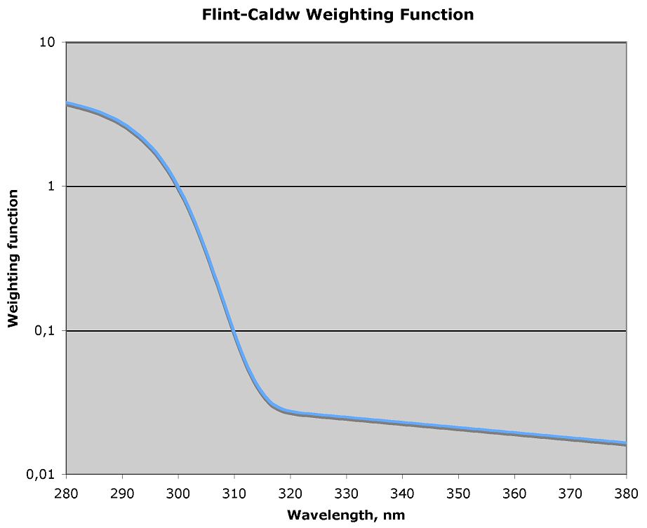{width="0.7\\myfigwidth"}
:::
Now you are ready to do the weighting itself. Select cells in column E
in rows corresponding to the values in the other columns. Select the
Calculator, and use it to multiply values in column B with the weighting
function. Select an empty cell and go a final time to the Calculator.
Select "Sum" and then the values you have just generated in column E.
The sum you get in the cell you selected is the weighted radiation
value. The number is, in this case, 0.000334759 and the unit is W
cm$^{-2}$, which can also be expressed as 3.35 . The bottom of the file
should look like Figure
[\[fig:Excel:sheet:bottom\]](#fig:Excel:sheet:bottom){reference-type="ref"
reference="fig:Excel:sheet:bottom"}. I have written $\Sigma$ in one cell
to remember that the value to the right of it is the sum of the values
above it.
::: figure*
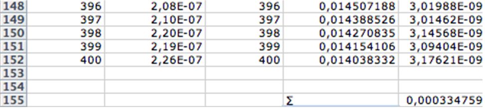{width="0.75\\myfigwidth"}
:::
Note that if you have another step size than 1 nm, you must multiply the
sum by that step size. It is recommended that you do not use step sizes
greater than 1 nm for UV-B spectra, since both the spectra themselves
and the weighting functions are so steep.
Martyn Caldwell's traditional Generalized Plant Action Spectrum is
easier to handle, and you should be able now to do a similar exercise
with it yourself. A formula for this weighting function has been
published by @Green1974: Weighting function
$= 2.618\cdot[1 -( \lambda/313.3)2]\cdot \exp[-(\lambda - 300)/31.08],$
where $\lambda$ stands for wavelength in nm. We abbreviate the name of
this action spectrum as GEN(G) elsewhere in this text. See section
[9.17](#app:formulations){reference-type="ref"
reference="app:formulations"} on page for the equations for other
commonly used BSWFs.
## Appendix: Calculation of effective doses with R {#app:R}
### Introduction {#introduction}
If you use the R system for statistics (see,
<http://www.r-project.org/>), or if you need an implementation with
fewer restrictions, you may want to use R instead of Excel to calculate
doses and action spectra. R is based on a real programming language
called S and allows much flexibility. We have developed a package to
facilitate these calculations. The package is called 'UVcalc' and will
be soon submitted to CRAN (Comprehensive R archive network) and will be
available also from this handbook's web page. In addition to functions
for calculating weighted and unweighted doses, and irradiance and from
energy irradiance spectra, also functions for calculating photon ratios
are provided.
### Calculating doses
Currently functions for five are implemented and are listed in Table
[\[tab:R:dose:functions\]](#tab:R:dose:functions){reference-type="ref"
reference="tab:R:dose:functions"}. The functions take two arguments one
vector giving the wavelengths and another vector giving the values of
spectral energy irradiance at these wavelengths. The spectral irradiance
or spectral exposure values would come either from measurements with a
spectroradiometer or from model simulations. All functions accept a
wavelengths vector with variable and arbitrary step sizes, with the
condition that the wavelengths are sorted in strictly increasing order,
something which is especially convenient when dealing with data from
array spectrometers[^31].
The functions are made available by installing the package `UVcalc`
(once) and loading it from the library when needed. To load the package
into the workspace use `library(UVcalc)`. Then load your spectral data
into R using `read.table()` or `read.csv()`.
A file from a Macam spectroradiometer starts:
``` {lastline="20"}
Wavelength(nm),W/m2
270,0
271,0
272,1.17E-04
273,2.42E-04
274,4.55E-04
275,8.94E-04
276,0.00161
277,0.00263
278,0.00412
279,0.00621
280,0.00904
281,0.01697
282,0.02069
283,0.02663
284,0.03314
285,0.04075
286,0.04895
287,0.05817
288,0.0679
```
For a file like this one, use the code below but replacing \"name\" with
the name and path to the data file. On Windows systems you need to scape
backslashes in file paths like this: '`\\`'.
{width="\\linewidth"}
If our spectral irradiance data is in , and the wavelength in nm, as in
the case of the Macam spectroradiometer, the functions will return the
effective irradiance in .
If, for example, the spectral irradiance output by our model or
spectroradiometer is in m, and the wavelengths are in Ångstrom then to
obtain the effective irradiance in we will need to convert the units.
{width="\\linewidth"}
In this example, we take advantage of the behaviour of the S language:
an operation between a scalar and vector, is equivalent to applying this
operation to each member of the vector. Consequently, in the code above,
each value from the vector of wavelengths is divided by 10, and each
value in the vector of spectral irradiances is divided by 1000.
If the spectral irradiance is in then values should be multiplied by 10
to convert them to .
It is very important to make sure that the wavelengths are in nanometers
as this is what the functions expect. If the wavelengths are in the
wrong units, the BSWF will be wrongly calculated, and the returned value
for effective irradiance will be wrong.
If we use as input to the functions instead of spectral irradiances,
time-integrated spectral irradiances in , then the functions will return
the effective exposure, or 'dose' in . Such time-integrated values are
more frequently available as the output of models, or by integrating
observed sequential values of spectral irradiance.
In addition to the functions for calculating biologically effective
doses and effective irradiances, we provide functions for calculating
unweighted doses or irradiances of (`PPFD()` or `PAR.q.dose()`, and
`PAR.e.dose()`), (`UVA.q.dose()` and `UVA.e.dose()`) and (`UVB.q.dose()`
and `UVB.e.dose()`), where 'e' variants return energy doses, and 'q'
variants return quantum or photon doses. All functions expect as input
radiation spectra in energy units, and wavelengths in nm.
### Calculating an action spectrum at given wavelengths
The functions available for calculating action spectra take as argument
a vector of wavelengths, and return a vector of effectiveness (either
quantum=photon or energy based) normalized to unity effectiveness at a
wavelength of 300 nm except when indicated. These functions are listed
in Table
[\[tab:R:action:spectra:functions\]](#tab:R:action:spectra:functions){reference-type="ref"
reference="tab:R:action:spectra:functions"}, and an example of their use
follows. In these examples we generate the wavelengths vectors in R, but
they can be also read from a file.
{width="\\linewidth"}
All functions accept a wavelengths vector with variable and arbitrary
step sizes, with the condition that the wavelengths are sorted in
strictly increasing order.
### Calculating photon ratios {#app:R:ratios:photon}
Functions are also provided for calculating photon ratios between
different pairs of wavebands. These functions are listed in Table
[\[tab:R:photon:ratios:functions\]](#tab:R:photon:ratios:functions){reference-type="ref"
reference="tab:R:photon:ratios:functions"}. We follow the most
frequently used wavelength ranges for the different colours, but also
provide some generic functions that can be used when other limits are
needed. Continuing with the example above in which my.data was read and
attached we calculate UV-B : PAR photon ratio
{width="\\linewidth"}
The spectral energy irradiance, can be in any energy based unit such as
, or , as the multipliers cancel out when calculating the ratio.
However, wavelengths must be always expressed in nanometers. Please, be
aware that these functions will return erroneous values if used with
spectra expressed as spectral photon irradiance, even though the
returned values are photon ratios.
Please, be aware that following common practice in the literature, the
wavelength range used for red light is different for the different
photon ratios.
### Documentation
The package includes manual pages for the different functions, and an
overview and a list of references for the original sources used. The
definition of the functions can bee seen once the package is loaded by
entering the name of the function without parameters or parentheses.
There are many resources on the R-System for Statistics and statistics
in general available on-line. The most useful ones are The R Wiki
(<http://rwiki.sciviews.org/>), and the documentation included in all R
installations and accompanying each one of the different packages.
Some classical books on R are those by @Dalgaard2002, @Crawley2005
[@Crawley2007], and @Venables2002. The book by [@Venables2000] discusses
programming in S, the language used in R to build new functions and
packages.
## Appendix: Suppliers of instruments {#sec:quant:suppliers}
In this section we provide names and web addresses to some suppliers of
instruments. This is certainly an incomplete list and exclusion reflects
only our ignorance.
**UV measurement:**\
<http://www.astranetsystems.com/>\
<http://www.avantes.com/>\
<http://www.bentham.co.uk/>\
<http://www.biosense.de/> ('*Viospore*' dosimeters.)\
<http://www.biospherical.com/>\
<http://www.deltaohm.com/>\
<http://www.delta-t.co.uk/>\
<http://www.gigahertz-optik.de/>\
<http://www.goochandhousego.com/> ('*Optronics*' spectroradiometers)\
<http://www.ictinternational.com.au/> (ELDONET terrestrial dosimeters)\
<http://www.intl-lighttech.com/>\
<http://www.irradian.co.uk/> ('*Macam*' instruments under new name)\
<http://www.kippzonen.com/>\
<http://www.oceanoptics.eu/>\
<http://www.roithner-laser.com/> (Photodiodes)\
<http://www.scitec.uk.com/>\
<http://www.sglux.com/> (SiC photodiodes, and instruments)\
<http://www.skyeinstruments.com/>\
<http://www.solarlight.com/>\
<http://www.spectralproducts.com/>\
<http://www.stellarnet.us/>\
<http://trios.de/> (RAMSES radiometers)\
<http://www.yesinc.com/> (Yankee Environmental Systems)\