---
title: "Flow of code execution"
subtitle: "R language constructs for flow control"
author: "Pedro J. Aphalo"
date: "2023-11-18"
date-modified: "2023-11-18"
format:
html:
mermaid:
theme: neutral
code-fold: show
keywords: [programming, webr-based]
callout-icon: false
engine: knitr
filters:
- webr
editor:
markdown:
wrap: 72
abstract: |
Interactive examples and flow chart diagrams for R language constructs for conditional evaluation and for repeated evaluation of code statements.
---
# Introduction
In a simple script the code statements are run (= executed, = evaluated)
one after another as they appear in the file, from top to bottom. A
simple script then always runs the same statements carrying out each
time the script is run the same computations.
This restriction is removed by including *control constructs* that based
on a test condition decide which code statement to run next. Using this
constructs we can make the computations done depend on data and their
properties. This is when programming starts being most useful or
"powerful", because the same code in scripts (or packages) becomes
useful with many different datasets.
We can group these constructs used to control the flow of code execution
from statement to statement in two groups: those that work as ON/OFF
switches and those that implement the repeated execution of a statement,
or *iteration*.
To make this work usefully, we need one more construct: a construct to
assemble a compound code statement from multiple simple code statements.
This makes it possible for the *control constructs* mentioned above to
control groups of statements or "chunks" of code in addition to simple
statements.
Below, we start with the sequential execution of statements in their
"natural" ordering and grouping into compound statements. Next, we look
and the ON/OFF or YES/NO constrtucts (`if`, `if ... else` and `ifelse`).
Last we look at the *iteration* or "repeated execution" *control
constructs* (`for ()`, `while()` and `repeat`).
::: callout-tip
# {{< bi keyboard-fill >}} Playgrounds or interactive R examples
Within this page you will run R examples in the web browser. You can
edit these code examples and run them again as many times as you like,
by clicking on the **Run Code** button above the 'WebR' text panels.
:::
# Unconditional execution
## Sequence
{fig-alt="A flow chart"
fig-align="center" width="25%"}
```{r}
a <- 123
b <- a * 2
print(b)
```
::: callout-tip
# {{< bi keyboard-fill >}} Playground
```{webr-r}
a <- 123
b <- a * 2
print(b)
```
:::
## Compound statement
{fig-alt="Flow chart showing two code statements enclosed within a box."
fig-align="center" width="30%"}
A group code statements enclosed in `{ }` conform a compoud statement.
By itself this construct does not modify the sequence in which
statements are executed or evaluated.
```{r}
a <- 123
{
  b <- a * 2
  print(b)
}
```
::: callout-tip
# {{< bi keyboard-fill >}} Playground
```{webr-r}
a <- 123
{
b <- a * 2
print(b)
}
```
:::
# Conditional execution
Decisions about which statement to run next are based on the result of a
test returning a `logical` value, TRUE`or`FALSE\`.
## `if ()` statement
{fig-alt="A flow chart showing two alternative paths downstream of a decision."
fig-align="center" width="67%"}
In an `if` statement, the decision is based on the value of a `logical`
vector of length one.
```{r}
a <- 123
if (a > 0) {
  print("'a' is positive")
}
print(a)
```
::: callout-tip
# {{< bi keyboard-fill >}} Playground
```{webr-r}
a <- 123
if (a > 0) {
print("'a' is positive")
}
print(a)
```
```{webr-r}
a <- c(1, 2, 3) # a vector of length 3
if (all(a > 0)) { # logical of length == 1
print("All 'a[i]' are positive")
}
print(a)
```
:::
## `if ()... else` statement
{fig-alt="Flow chart with two paths downstream of the decision."
fig-align="center" width="95%"}
```{r}
a <- 123
if (a >= 0) {
  print("'a' is positive")
} else {
  print("'a' is negative")
}
print(a)
```
::: callout-tip
# {{< bi keyboard-fill >}} Playground
```{webr-r}
a <- 123
if (a >= 0) {
print("'a' is positive")
} else {
print("'a' is negative")
}
print(a)
```
For dealing with vectors longer that one we can use `all()` and `any()`.
Of course, if they describe the decision we need to process our data.
```{webr-r}
a <- c(1, 2, 3) # a vector of length 3
if (all(a > 0)) { # logical of length == 1
print("All 'a[i]' are positive")
} else {
print("One or more 'a[i]' are negative")
}
print(a)
```
An advanced/more sophisticated alternative is to count the number of
members in the vector that are positive and negative.
```{webr-r}
a <- c(1, 2, 3) # a vector of length 3
if (all(a >= 0)) {
print("All 'a[i]' are positive")
} else if (all(a < 0)) {
print("All 'a[i]' are negative")
} else {
print(paste("'a' contains",
sum(a >= 0), "positive and",
sum(a < 0), "negative values."))
}
print(a)
```
:::
## `switch` statement
In a switch statement the decision selects the evaluation of one among
multiple alternative staements. The "selector" can be an integer or a
character vector of length equal to one.
{fig-alt="Flow chart with multiple parallel paths for evaluation."
fig-align="center" width="80%"}
Using names for the _cases_ in the switch.
```{r}
my.char <- "two"
my.fraction <- switch(my.char,
                      one = 1,
                      two = 1 / 2,
                      four = 1 / 4,
                      0
)
print(my.fraction)
```
::: callout-tip
# {{< bi keyboard-fill >}} Playground
```{webr-r}
my.char <- "two"
my.number <- switch(my.char,
one = 1,
two = 2,
four = 4,
0
)
print(my.number)
```
```{webr-r}
my.char <- "dos"
my.number <- switch(my.char,
one =, uno = 1,
two =, dos = 2,
four =, cuatro = 4,
0
)
print(my.number)
```
:::
Using numbers to select cases by position.
::: callout-tip
# {{< bi keyboard-fill >}} Playground
```{webr-r}
my.number <- 2
my.char <- switch(my.number,
"one",
"two",
"three", # needed!!
"four",
"not one, two or four"
)
print(my.char)
```
:::
## `ifelse(...)` *vectorised* statement
Function `ifelse()` works very differently than `if () ... else`. The
decision can, and in most cases, it is based on a long logical vector.
The returned value has the same length as the `logical` vector.
```{r}
a <- c(1, 2, -1, 3) # a vector of length 3
ifelse(a >= 0, "positive", "negative")
print(a)
```
::: callout-tip
# {{< bi keyboard-fill >}} Playground
```{webr-r}
a <- 123
ifelse(a >= 0, "positive", "negative")
print(a)
```
```{webr-r}
a <- c(1, 2, -1, 3)
ifelse(a >= 0, "positive", "negative")
print(a)
```
:::
# Iteration or repeated execution
## `for ()` statement
{fig-alt="Flow chart showing a closed execution path with an entry and an exit."
fig-align="center" width="70%"}
In a `for` statement, the controlled statement is run with one member of
a list or vector at a time, normally walking from "head" to "tail" of
the list or vector. The value of each member is accessed through a
"place holder" variable. The name of the arbitrary variable can be any
valid R name.
```{r}
a <- c(1, 2, -1, 3)
for (a_member in a) {
  print(a_member)
}
print(a)
```
::: callout-tip
# {{< bi keyboard-fill >}} Playground
```{webr-r}
a <- c(1, 2, -1, 3)
for (a_member in a) {
print(a_member)
}
print(a)
```
Using extraction operator `[ ]` and indexing.
```{webr-r}
a <- c(1, 2, -1, 3)
sum_of_a <- 0
for (i in seq_along(a)) {
sum_of_a <- sum_of_a + a[i]
print(sum_of_a)
}
print(a)
```
We can end early.
```{webr-r}
a <- c(1, 2, -1, 3)
for (a_member in a) {
if (a_member < 0) {
break()
}
print(a_member)
}
print(a)
```
We can jump to the next.
```{webr-r}
a <- c(1, 2, -1, 3)
for (a_member in a) {
if (a_member < 0) {
next()
}
print(a_member)
}
print(a)
```
:::
## `while()` statement
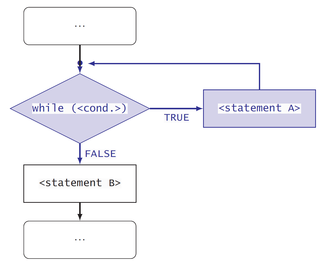{fig-alt="Flow chart with a closed loop with an entry and an exit point."
fig-align="center" width="70%"}
```{r}
a <- c(1, 2, -1, 3)
i <- 0
sum_of_a <- 0
while(i < length(a)) {
  i <- i + 1
  sum_of_a <- sum_of_a + a[i]
  print(sum_of_a)
}
print(i)
```
::: callout-tip
# {{< bi keyboard-fill >}} Playground
```{webr-r}
a <- c(1, 2, -1, 3)
i <- 0
sum_of_a <- 0
while(sum_of_a < 2) {
i <- i + 1
sum_of_a <- sum_of_a + a[i]
print(sum_of_a)
}
print(i)
```
```{webr-r}
a <- c(1, 2, -1, 3)
i <- 1
sum_of_a <- 0
while(sum_of_a < 2) {
sum_of_a <- sum_of_a + a[i]
print(sum_of_a)
i <- i + 1
}
print(i)
```
:::
## `repeat` statement
{fig-alt="Flow chart with a loop with an exit point at an arbitrary point within the loop."
fig-align="center" width="70%"}
```{r}
a <- c(1, 2, -1, 3)
i <- 0
sum_of_a <- 0
while(i < length(a)) {
  i <- i + 1
  sum_of_a <- sum_of_a + a[i]
  print(sum_of_a)
}
print(i)
```
::: callout-tip
# {{< bi keyboard-fill >}} Playground
```{webr-r}
a <- c(1, 2, -1, 3)
i <- 0
sum_of_a <- 0
repeat {
if (sum_of_a >= 2) {
break()
}
i <- i + 1
sum_of_a <- sum_of_a + a[i]
print(sum_of_a)
}
print(i)
```
```{webr-r}
a <- c(1, 2, -1, 3)
i <- 1
sum_of_a <- 0
repeat {
sum_of_a <- sum_of_a + a[i]
print(sum_of_a)
if (sum_of_a >= 2) {
break()
}
i <- i + 1
}
print(i)
```
:::
# Take home message
Now you know all the important constructs that make it possible to control the flow of evaluation of statements in a script or program. With small variations in their syntax, these same constructs are available in many different computer programming languages.
That all these constructs are available in R, makes of R a proper programming language. **It also means that learning to program in additional computer languages is much easier than learning the first one.**


